Comparison of scanning aerosol lidar and in situ measurements of aerosol physical properties and boundary layer heights

The spatiotemporal distribution of aerosol particles in the atmosphere has a great impact on radiative transfer, clouds, and air quality. Modern remote sensing methods, as well as airborne in situ measurements by unpiloted aerial vehicles (UAV) or balloons, are suitable tools to improve our understanding of the role of aerosol particles in the atmosphere. To validate the measurement capabilities of three relatively new measurement systems and to bridge the gaps that are often encountered between remote sensing and in situ observation, as well as to investigate aerosol particles in and above the boundary layer, we conducted two measurement campaigns and collected a comprehensive dataset employing a scanning aerosol lidar, a balloon-borne radiosonde with the Compact Optical Backscatter Aerosol Detector (COBALD), an optical particle counter (OPC) on a UAV, and a comprehensive set of ground-based instruments. The extinction coefficients calculated from near-ground-level aerosol size distributions measured in situ are well correlated with those retrieved from lidar measurements, with a slope of 1.037 ± 0.015 and a Pearson correlation coefficient of 0.878, respectively. Vertical profiles measured by an OPC-N3 on a UAV show similar vertical particle distributions and boundary layer heights to lidar measurements. However, the sensor, OPC-N3, shows a larger variability in the aerosol backscatter coefficient measurements, with a Pearson correlation coefficient of only 0.241. In contrast, the COBALD data from a balloon flight are well correlated with lidar-derived backscatter data from the near-ground level up to the stratosphere, with a slope of 1.063 ± 0.016 and a Pearson correlation coefficient of 0.925, respectively. This consistency between lidar and COBALD data reflects the good data quality of both methods and proves that lidar can provide reliable and spatial distributions of aerosol particles with high spatial and temporal resolutions. This study shows that the scanning lidar has the capability to retrieve backscatter coefficients near the ground level (from 25 to 50 m above ground level) when it conducts horizontal measurement, which is not possible for vertically pointing lidar. These near-ground-level retrievals compare well with ground-level in situ measurements. In addition, in situ measurements on the balloon and UAV validated the scanning lidar retrievals within and above the boundary layer. The scanning aerosol lidar allows us to measure aerosol particle distributions and profiles from the ground level to the stratosphere with an accuracy equal to or better than in situ measurements and with a similar spatial resolution.

1 Introduction

The large varieties of aerosol spatiotemporal distributions in the atmosphere cause large uncertainties in radiative forcing globally (Ramanathan et al., 2001), and these uncertainties have a great impact on climate change simulations (IPCC, 2014). The distributions and evolution of aerosol are related to the emission of aerosols (Grythe et al., 2014; Tegen and Schepanski, 2018; Hamilton et al., 2022) and their loss pathway (Poreh and Cermak, 1964; Cheng et al., 2011; Xiang et al., 2019; Xue et al., 2022). In addition, another important factor affecting radiative forcing is aerosol optical properties (e.g., single-scattering albedo (SSA), lidar ratio, scattering, and absorption coefficients) (Alam et al., 2011; Romshoo et al., 2021), which also have large varieties for different types of aerosols (Lesins et al., 2002; Floutsi et al., 2023).

Many methods have been used to measure the spatiotemporal distribution of aerosol optical parameters regionally and globally. One of the most successful instruments for this purpose is the Moderate Resolution Imaging Spectroradiometer (MODIS) on the Terra and Aqua satellites (Filonchyk and Hurynovich, 2020; Qin et al., 2021). MODIS can provide column-integrated optical parameters like aerosol optical depth (AOD), Ångström exponent (AE), and single-scattering albedo (SSA) to study the optical properties of mineral dust (Kaufman et al., 2005; Ginoux et al., 2012), urban aerosol (More et al., 2013; Munchak et al., 2013), forest fire smoke (Maeda et al., 2009; Huesca et al., 2009), and so on. Another successful satellite mission is the Cloud–Aerosol Lidar and Infrared Pathfinder Satellite Observations (CALIPSO). CALIPSO combines an active lidar instrument with passive infrared and visible images to probe the vertical structure and properties of thin clouds and aerosols across the globe (Winker et al., 2009; Wang et al., 2021; Salehi et al., 2021; Tesche et al., 2014). China launched its first spaceborne aerosol–cloud high-spectral-resolution lidar (ACHSRL), on 16 April 2022, which is capable of high-accuracy profiling of aerosols and clouds around the globe (Ke et al., 2022). Also, the Earth Cloud, Aerosol, and Radiation Explorer (EarthCARE) is a satellite mission implemented by the European Space Agency (ESA), in cooperation with the Japan Aerospace Exploration Agency (JAXA), to measure global profiles of aerosols, clouds, and precipitation properties, together with radiative fluxes and derived heating rates, and is due for launch in May 2024 (Wehr et al., 2023).

In addition to these satellite missions, ground-based remote sensing methods are used to investigate aerosol optical properties (Adam et al., 2020; Mylonaki et al., 2021). Over the last few decades, many ground-based observation networks were established to investigate aerosol properties regionally and globally. For example, the AERONET (AErosol RObotic NETwork) project is a federation of ground-based remote sensing aerosol networks that provides globally distributed observations of spectral aerosol optical depth (AOD), inversion products, and precipitation water in diverse aerosol regimes (Holben et al., 1998; Prasad and Singh, 2007; Mielonen et al., 2009). The MicroPulse Lidar Network (MPLNET) is a federated network of the MicroPulse Lidar (MPL) systems designed to measure aerosol and cloud vertical structure and boundary layer heights (Welton et al., 2006; Lolli et al., 2018). The European Aerosol Research Lidar Network (EARLINET) is a multi-wavelength lidar network designed to create a quantitative, comprehensive, and statistically significant database for the horizontal, vertical, and temporal distribution of aerosols on a continental scale (Pappalardo et al., 2014; Marinou et al., 2017).

Aerosol elastic scattering lidar is widely used in lidar observation networks as it can provide detailed information with high spatial and temporal resolution. However, retrieving backscatter coefficients from this kind of lidar data requires assumptions of lidar ratios and reference values (Fernald, 1984; Klett, 1985). One of the successfully used technologies to overcome this problem is the Raman lidar (Wandinger, 2005; Groß et al., 2015; Baars et al., 2016; Hu et al., 2022). Another widely used technology is the high-spectral-resolution lidar (HSRL) (Liu et al., 1999) which used a narrowband filter (e.g., atom or molecule filter) to separate signals from molecule and particle backscattering (Piironen and Eloranta, 1994). And this HSRL allows us to better investigate aerosol optical properties (Burton et al., 2012, 2014; Groß et al., 2013). Recently, a HSRL that uses an interferometer as a filter has been deployed at other wavelengths. The recently launched Doppler wind lidar, ALADIN, uses this technology to measure tropospheric wind profiles on a global scale but can also obtain vertical aerosol profiles (Schillinger et al., 2003).

In situ measurements can also help us better understand aerosol optical properties. The most common instruments are the nephelometer and Aethalometer, which can measure the wavelength-dependent optical parameters like scattering and absorption coefficients of aerosol particles (Anderson et al., 1996; Zieger et al., 2011; Drinovec et al., 2015). The aerosol optical parameters are determined by particle size distribution, particle shape, and complex refractive index (Bohren and Huffman, 2008; Yao et al., 2022). The size distribution can be measured by different kinds of particle sizers like the scanning mobility particle sizer (SMPS), optical particle counter (OPC), and aerodynamic particle sizer (APS). The aerosol complex refractive index is related to the aerosol chemical composition which can be measured by aerosol mass spectrometry, as well as the relative humidity (Zieger et al., 2015). For decades, these in situ aerosol characterization instruments not only provided valuable datasets at ground level (Huang et al., 2019; Jiang et al., 2022) but also were deployed on aircraft, balloons, mountains (Zieger et al., 2012), and unpiloted aerial vehicles to get vertical profiles of aerosol parameters (Bahreini et al., 2003; Zhen et al., 2018; Brunamonti et al., 2021).

Although many results have reported aerosol measurements by lidar (Matthias and Bösenberg, 2002; Pappalardo et al., 2014; Hofer et al., 2020), there are fewer reports on the comparison of in situ measurement with lidar measurement to quantify the uncertainties in the lidar retrievals (Xiafukaiti et al., 2020; Düsing et al., 2018). In addition, most vertically pointing lidar systems have overlap gap between the detector's field of view and the laser beam from tens of meters to around 1000 m, which makes it difficult to get valid measurement near the surface (Wandinger and Ansmann, 2002) to compare with ground-level in situ measurements. However, scanning lidar can conduct horizontal measurements, allowing us to get vertical profiles of the aerosol particles and boundary layer structure near the ground level (Althausen et al., 2000). In addition, scanning aerosol lidar can also determine lidar ratios to reduce the uncertainties in the lidar retrievals (Fernald, 1984; Zhang et al., 2022).

In recent years, vertical profiles of aerosol have also been investigated more and more by unpiloted aerial vehicles (UAVs) and lidar. For example, Liu et al. (2020) used the UAVs and lidar to study the vertical distribution of PM_2.5 and interactions with the atmospheric boundary layer during the development of heavy haze pollution. Ferrero et al. (2019) compared the backscatter coefficient retrieved from lidar with that calculated from aerosol size distributions measured by OPC on tethered balloons in the Arctic to study the role of aerosol chemistry and dust composition in a closure experiment. Zhang et al. (2021) compared boundary layer heights retrieved from aerosol lidar and tethered balloon measurements in semi-arid regions. Liu et al. (2021) found that the wind shear generating turbulence reshaped the vertical profiles of parameters such as potential temperature (θ) and PM_2.5 in the nocturnal boundary layer, which was the key factor leading to the development of entrainment at nighttime. Reineman et al. (2016) used ship-launched fixed-wing UAVs to measure the marine atmospheric boundary layer and ocean surface processes. In addition, the vertical profiles of atmospheric parameters related to aerosol process such as temperature (Zarco-Tejada et al., 2012), relative humidity (Spiess et al., 2007), wind (Spiess et al., 2007), and ozone concentration (Guimarães et al., 2019) are also obtained from UAV flights.

However, to our best knowledge, so far no dedicated comparison of scanning lidar measurement with in situ observation has been performed over a wide altitude range and over such a long time period for comparison at ground level (e.g., 1-month dataset with 10 min resolution). Also, in order to bridge the gaps that are often encountered between remote sensing and in situ observation, we compared datasets on aerosol spatiotemporal distributions and evolution by combining remote sensing and in situ measurements. Two field campaigns were conducted that employed a scanning aerosol lidar, a radiosonde with a backscatter sensor, an OPC on a UAV, and a comprehensive set of ground-level instruments. The first field campaign was conducted in downtown Stuttgart to compare lidar retrievals with ground-level in situ measurements. The second field campaign was done at the Jülich Research Center to compare lidar retrievals with OPC measurements on a UAV and a Compact Optical Backscatter Aerosol Detector (COBALD) backscatter sensor on a radiosonde. The aim of this work is to compare the different methods in aerosol measurements, to validate scanning lidar retrievals, and to discuss the uncertainties in the different methods and the boundary layer evolutions from lidar and UAV retrievals.

2 Methods

Two field campaigns were conducted in downtown Stuttgart and at Jülich Research Center to compare scanning aerosol lidar measurements with different in situ measurements. The first field campaign was conducted from 5 February to 5 March 2018 in downtown Stuttgart (48.7986° N, 9.2024° E; 247 m above sea level) by employing a mobile container and a scanning aerosol lidar on the roof of the container. The ground-level in situ measurements deployed in this mobile container provided aerosol particle size distributions, aerosol chemical composition, and meteorological information (Huang et al., 2019). The second field campaign was conducted from 5 to 12 July 2018 at Jülich Research Center (50.9084° N, 6.4131° E; 110 m above sea level) by employing a scanning aerosol lidar, a COBALD sensor hosted by a Vaisala RS41-SGP radiosonde, and an OPC on a UAV. The scanning lidar, called KASCAL (Karlsruhe scanning aerosol LiDAR), used in these two field campaigns was developed by Raymetrics (LR111-ESS-D200, Raymetrics). A UAV (eBee, senseFly) carrying one OPC (OPC-N3, Alphasense UK), weather sensors, and global positioning system (GPS) sensors provided altitude-dependent particle size distribution and also meteorological information above the Jülich Research Center. In addition, atmospheric parameters like pressure, temperature, relative humidity, and wind information from the ground to 30 km above Jülich Research Center were gathered by a GPS-equipped radiosonde aboard a balloon that carried COBALD to measure altitude-dependent in situ backscatter coefficients at two wavelengths (455 and 940 nm) (Brunamonti et al., 2021). The measurements during this work indicated that the backscatter was dominated by smaller particles with low-depolarization ratios so that it seemed justified to use a spherical model to represent these aerosol particles (Khlebtsov et al., 2005; Moroz, 2009; Wang et al., 2023). Hence, a Mie code (Leinonen, 2016) was used to calculate extinction coefficients and backscatter coefficients from aerosol size distributions for comparison with the lidar retrieval.

2.1 Scanning aerosol lidar

The 3D scanning lidar (KASCAL) used in the above two field campaigns has an emission wavelength of 355 nm and is equipped with elastic, depolarization, and vibrational Raman channels, hence allowing us to retrieve extinction coefficients, backscatter coefficients, and depolarization ratios. The laser pulse energy and repetition frequency are 32.1 mJ and 20 Hz, respectively. The laser head, 200 mm telescope, and lidar signal detection units are mounted on a rotating platform that allows zenith angles from −7 to 90° and azimuth angles from 0 to 360°. This lidar works automatically, is time-controlled, and works continuously via software developed by Raymetrics. Detailed information can be found at https://www.raymetrics.com/product/3d-scanning-lidar (last access: 8 March 2021) (Avdikos, 2015; Zhang et al., 2022). During the first field campaign in downtown Stuttgart, the lidar conducted zenith scans with an elevation angle from 90 to 5° in steps of 5°. The measurements at 5° were used over a range representative of an altitude of 25–50 m to compare with ground-level in situ measurements (3.7 m above ground level). It is assumed that these values are comparable within the mixing layer. During the second field campaign at Jülich Research Center, the lidar conducted zenith scans during a UAV launch, and the measurements at all elevation angles were used to get vertical profiles of aerosols from the ground level up to the free troposphere to compare with an OPC measurement on the UAV. In addition, the lidar also conducted vertical-pointing measurements during the night of 12 July 2018 at Jülich Research Center to compare the vertical profiles of backscatter coefficients from lidar retrievals and COBALD measurement aboard a radiosonde.

For the data analysis and calibration of the lidar system, we followed the quality standards of EARLINET (Freudenthaler, 2016). For data analysis of zenith scans, we determined the vertical backscatter coefficient profiles using the Klett–Fernald method (Fernald, 1984; Klett, 1985). And these vertical profiles of aerosol backscatter coefficients were used as the reference values for other observation angles. In addition, the measured temperatures and pressures from UAVs and balloons were used to calculate the molecular backscatter coefficients which can be used in lidar retrievals.

The atmospheric boundary layer height can be determined from lidar using the Haar wavelet transform (HWT) method (Baars et al., 2008). Furthermore, the boundary layer height was retrieved from vertical profiles of potential temperature using the gradient method (Seidel et al., 2010; Li et al., 2021).

2.2 Ground-level in situ measurements in downtown Stuttgart

The ground-level in situ instruments were deployed in a mobile container that was deployed in a park in downtown Stuttgart. Ambient temperature, relative humidity, wind direction, wind speed, global radiation, pressure, and precipitation data were measured by a meteorological sensor (WS700, G. Lufft Mess- und Regeltechnik GmbH). Trace gases (O₃, CO₂, NO₂, and SO₂) were measured with the gas monitors (Environnement S.A). Particle number concentrations were recorded with two condensation particle counters (CPCs 3774 and 3022, TSI Incorporated,). Particle size distributions were measured with SMPS (differential mobility analyzer (DMA) – TSI 3080, TSI Incorporated; CPC – CPC3022, TSI Incorporated) and OPC (Fidas200, Palas GmbH). The OPC (Fidas200, Palas GmbH) continuously measured particles in the size range of 0.18–18 µm. The OPC used the Lorenz–Mie theory to determine the particle number size distribution, and this size distribution can be used to calculate extinction coefficients via a Mie code (Leinonen, 2016). In this experiment, Fidas200 was operated with a flow rate of 5 L min⁻¹ and with a time resolution of 1 s.

Figure 1 shows the workflow used to derive the aerosol extinction coefficients from Mie calculations based on in situ aerosol characterization instruments. The aerosol sizer (e.g., OPC) can provide a dry aerosol particle size distribution which can be converted to the ambient aerosol size distributions using hygroscopic growth factors (κ) calculated from aerosol chemical composition using the ISORROPIA II thermodynamic equilibrium model (Fountoukis and Nenes, 2007). The aerosol chemical composition was measured by high-resolution time-of-flight aerosol mass spectrometer (HR-ToF-AMS) (Aerodyne Research Inc.). As most aerosol particles are constrained and well mixed within the boundary layer, the aerosol complex refractive index remains almost constant (Raut and Chazette, 2008). Although the Sun photometer is integrating over the whole vertical column, the relatively high aerosol concentrations in the boundary layer dominate (Li et al., 2017). Therefore, it seems justified to use the aerosol complex refractive index derived from a nearby Sun photometer (CE-318). Hence, we used the aerosol complex refractive index derived from a nearby Sun photometer (CE-318). With ambient aerosol size distribution and complex refractive index, optical parameters (e.g., extinction coefficients) were calculated to compare with lidar retrievals.

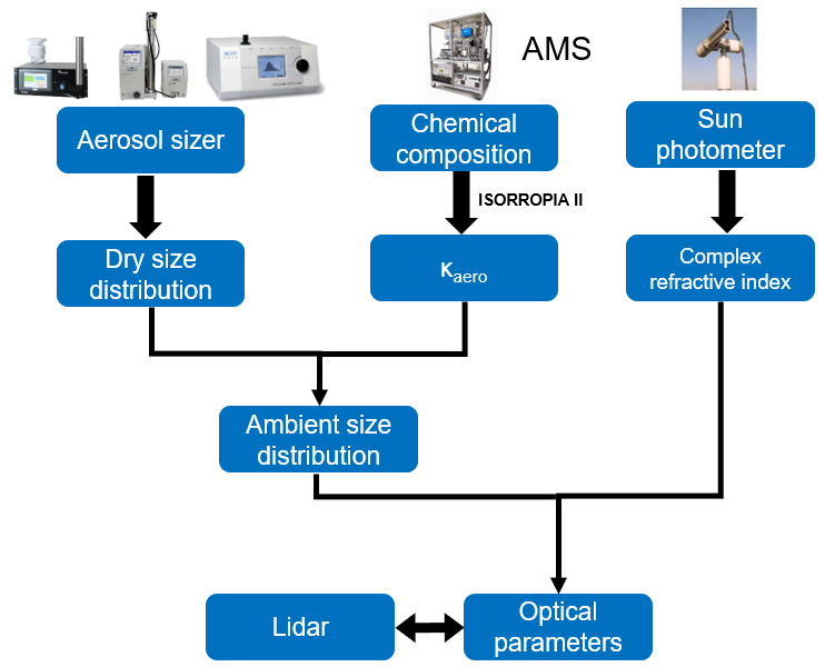
Figure 1 Process flow in deriving aerosol extinction coefficients from the Mie calculation and parameters used in Mie calculations. κ_aero is the composition-dependent hygroscopicity growth factor.

2.3 UAV and balloon-borne measurements at Jülich Research Center

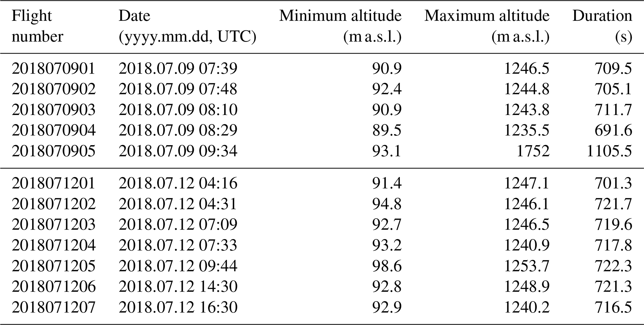
Data of an OPC (OPC-N3, Alphasense UK) on a UAV and a COBALD backscatter sensor (Institute for Atmospheric and Climate Science, ETH Zürich) on a balloon were collected at Jülich Research Center in July 2018. The UAV used in this field campaign is a fixed-wing drone (eBee, senseFly) which is operated by the Institute of Energy and Climate Research – Troposphere (IEK-8). Its payload is 320 g at a total weight of 750 g, with the highest observation altitude of approximately 1200 m above ground level. The ascent and descent velocity of this UAV was around 3.2 m s⁻¹. The measurement sensors were mounted inside the UAV. The size distributions were measured in real time with a time resolution of 1.6 s by OPC-N3. Additionally, atmospheric parameters such as air temperature, air pressure, relative humidity, wind speed, and wind direction were measured with a temporal resolution of 1 s. The UAV was launched five times during the morning from 07:00 to 10:00 UTC​​​​​​​ on 9 July to measure the boundary layer dynamics in the early morning and was launched seven times from 03:50 to 16:30 UTC on 12 July to measure the boundary layer transition from nocturnal boundary layer to the mixing layer. The detailed UAV fights information can be found in Table 1.

Table 1 Time, altitude, and duration of UAV flights for the experiments on 9 and 12 July 2018.

Besides, a radiosonde balloon which was operated by the Institute of Energy and Climate Research – Stratosphere (IEK-7) measured the atmospheric parameters from the ground to 25 km altitude. COBALD was part of a CFH (water vapor)/ECC (ozone) ozone/RS41 payload to provide the backscatter coefficients, as well as air temperature, air pressure, relative humidity, wind, and ozone concentration, with the temporal and spatial resolution being 1 s and about 5 m vertically.

(Smit et al., 2007)20072016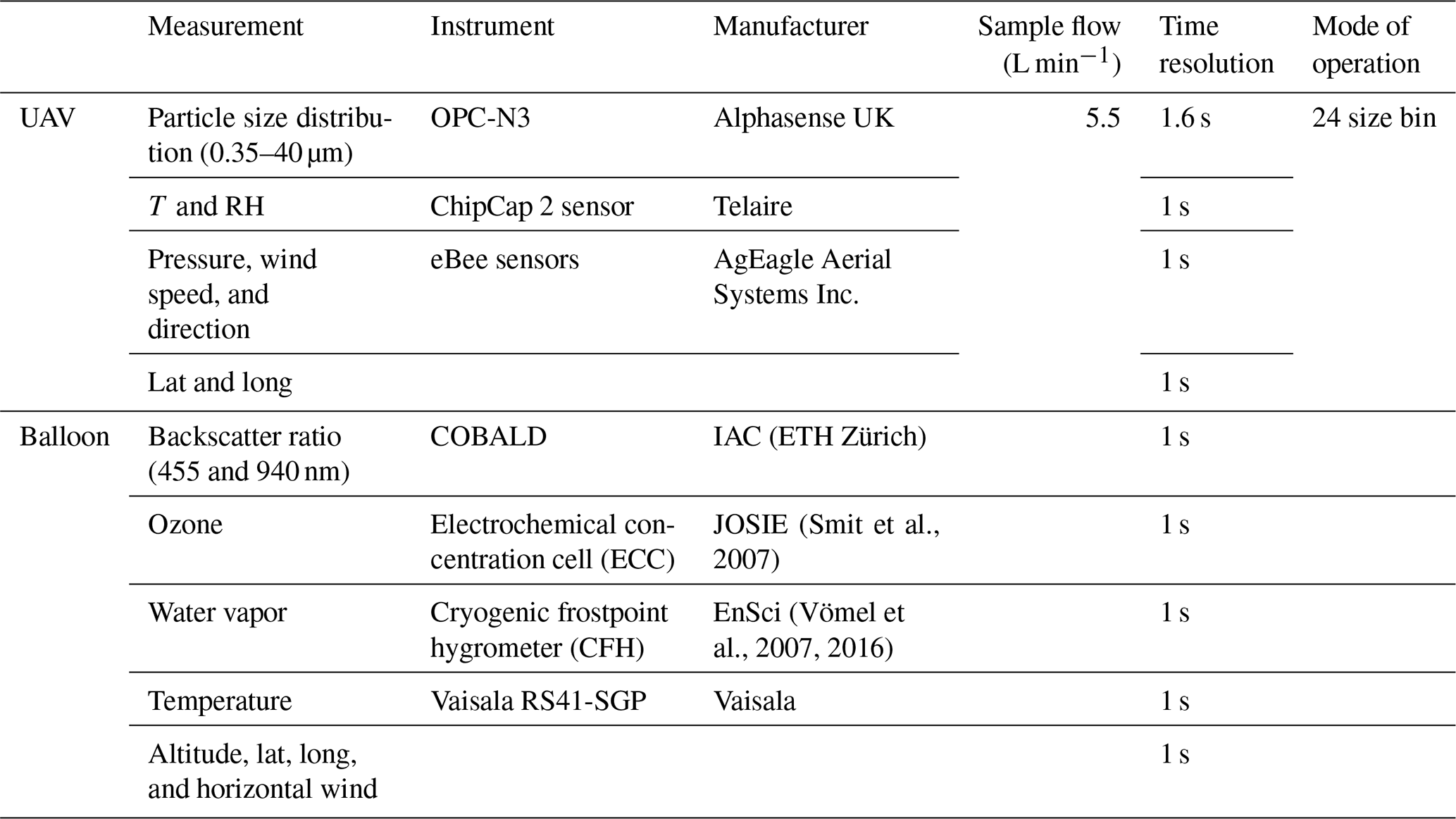

Table 2 Summary of sensors used on UAV and balloon fights.

COBALD is a lightweight (500 g) aerosol backscatter detector for balloon-borne measurements developed at the Institute for Atmospheric and Climate Science (ETH Zürich), based on the original approach by Rosen and Kjome (1991). Two light-emitting diodes (LEDs) as light sources and a photodiode detector with a field of view (FOV) of 6° provide high-precision in situ measurements of aerosol backscatter at wavelengths of 455 nm (blue visible) and 940 nm (infrared). COBALD has been originally developed for the observation of high-altitude clouds, such as cirrus (Brabec et al., 2012; Cirisan et al., 2014) and polar stratospheric clouds (Engel et al., 2014), while recently it was proven able to detect and characterize aerosol layers in the upper troposphere–lower stratosphere (Vernier et al., 2015, 2018; Brunamonti et al., 2018, 2021). In this work, we compared COBALD measurements with scanning aerosol lidar measurements for validating lidar retrievals and investigating the vertical distribution of aerosols. A summary of sensors used on UAV and balloon fights is shown in Table 2.

3 Results and discussion

3.1 Comparison of lidar data with ground-level in situ measurements

The comparison of lidar retrievals with ground-level aerosol sizer data was conducted during a field campaign from 5 February to 5 March 2018 in downtown Stuttgart. In this campaign, the aerosol lidar did zenith scans with an elevation angle from 90 to 5° in steps of 5°. The nearly horizontal measurement at 5° allows us to retrieve extinction coefficients near ground level (from 25 to 50 m above ground level) using short-range lidar data (ranges from 285 to 570 m) that can be compared with the ground-level in situ measurements (sampled 3.7 m above ground level). The ground-level in situ aerosol sizer, Fidas200, measured the aerosol size distributions which were used to calculate the aerosol extinction coefficients via Mie code. Figure 2 shows the extinction coefficients retrieved from lidar measurements and from Mie calculations based on aerosol size distribution (labeled as “Raw size distribution”). The extinction coefficients obtained from lidar were both retrieved from the slope and Raman retrieval methods (Seidel et al., 2010; Ansmann et al., 1992). In the slope and Raman retrieval methods, a linear regression was used, and the correlation coefficients of linear regressions are 0.99 ± 0.05 and 0.99 ± 0.06 for slope and Raman retrieval methods, respectively. This is also an indication of a rather homogeneous distribution of the aerosol particles within the altitude range from 25 to 50 m corresponding to a range between 285 and 570 m. This figure shows that the extinction coefficients from Mie calculations based on raw OPC size distributions are systematically lower than those from lidar retrievals by a factor of 4.70 ± 1.49. The reason for this phenomenon is that the Fidas200 underestimates the particle number by a factor of 2–10 at diameters between 0.25 and 0.5 µm when compared with SMPS data as shown in Fig. S1 in the Supplement. The left-hand side of Fig. S1 shows the number size distribution from Fidas200 and the merged size distribution from SMPS and APS measurements. The right plot of Fig. S1 shows the accumulated extinction coefficients calculated from Mie theory based on those two size distributions, which shows the substantial difference by a factor of 4. Hence, we conclude that the underestimation of particle numbers from 0.25 to 0.5 µm is one of the main reasons for the underestimation of extinction coefficients based on uncorrected OPC data.

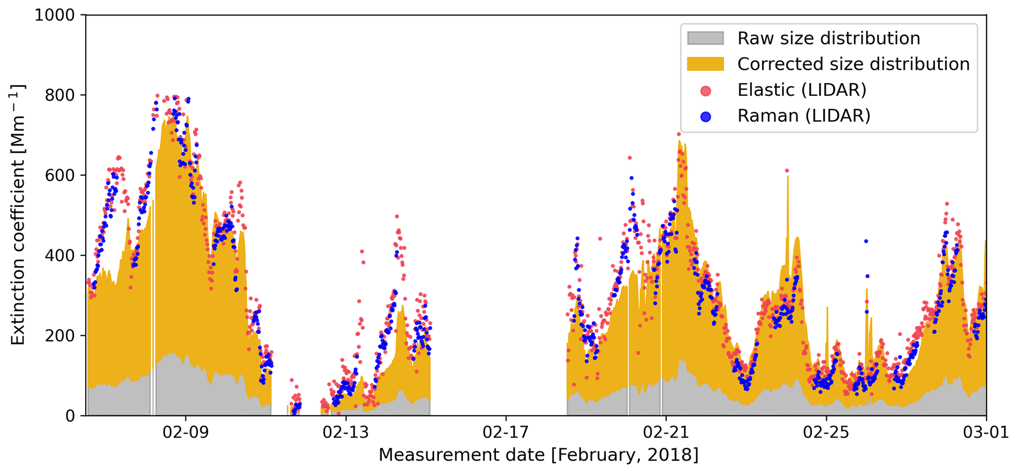
Figure 2 Time series of ground-level extinction coefficients retrieved from lidar measurements (both elastic and Raman methods) and from Mie calculations based on OPC raw size distributions, as well as size distributions corrected by counting efficiency from 5 February to 5 March 2018 in downtown Stuttgart.

Based on systematic laboratory measurements with the different particle sizers Fidas200 OPC, SMPS, and APS the FIDAS200 counting efficiency was determined (see Fig. S2). This counting efficiency was used to correct all measured size distributions. The corrected size distributions were used to calculate the extinction coefficients via Mie calculation. The time series of the extinction coefficients calculated from the corrected size distribution is shown in Fig. 2 (orange area). The calculated extinction coefficients show a reasonable agreement with the lidar retrievals.

The correlation plot between the extinction coefficient from Fidas200 and the lidar-derived extinction coefficient is shown in Fig. 3, which shows a slope and a Pearson correlation coefficient of 1.037 ± 0.015 and 0.878, respectively. As shown in Fig. 2, the extinction coefficients retrieved from the lidar measurement show a similar trend to those calculated based on corrected Fidas200 size distributions. Please note that the extinction coefficient based on Fidas200 data is still a little lower than those based on lidar measurements. This may be caused by a partial loss of water from the aerosol particles due to higher temperatures inside the container. However, the aerosol particles are not expected to reach equilibrium within the residence time of 3 s in the sampling line inside the warm container. Please note that there was no dryer in the sampling line. From the fraction of extinction coefficients shown in Fig. 2, we can determine that the main reason for causing extinction coefficient inconsistency between in situ measurement and lidar retrieval is undercounting by Fidas200. The relatively good agreement of the extinction coefficients after our reasonable corrections reflects the reliability of our methods and the good quality of the lidar retrievals.

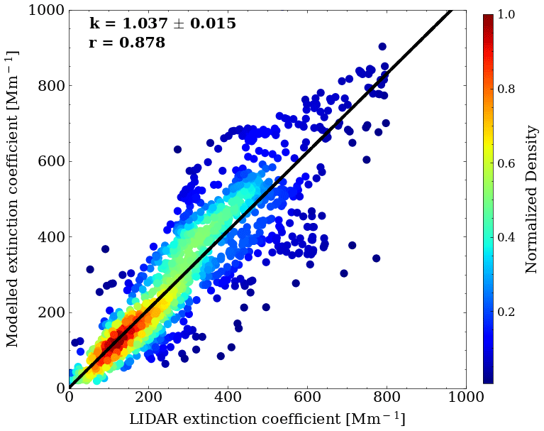
Figure 3 Correlation of extinction coefficients from lidar retrieval and Mie calculation from 5 February to 5 March 2018 in Stuttgart. The relative humidity used in the model is a container for indoor relative humidity, and the black line is the regression fitting curve of them. The red line is the regression fitting curve between the lidar-derived extinction coefficients and those from Mie calculation using ambient relative humidity.

3.2 Comparison of lidar data with in situ measurements on a UAV

The comparison of lidar and UAV measurements was conducted for 2 d on 9 and 12 July 2018 to study the vertical distribution of aerosols and the boundary layer structure. The sky was almost free of clouds during UAV flights on 9 July, while it was affected by clouds within the boundary layer on 12 July.

Figure 4 shows the time series of backscatter coefficients, boundary layer heights (pink squares), and residual layer heights (yellow squares) retrieved from lidar measurement (pink squares), as well as boundary layer heights (a.s.l. – above see level) obtained from UAV measurements (black star with a white circle surrounding it) and from ERA5 dataset (dashed white line) on 9 July 2018. This figure shows that the boundary layer height retrieved from the lidar measurement is consistent with the boundary layer height from the UAV measurement for which both show an increasing trend in the boundary layer during the morning of this day. In addition, the boundary layer from ERA5 also shows a similar trend to the observations but overestimates boundary layer height, especially during daytime. A possible reason for this overestimation is that the existence of clouds during the daytime reduced solar radiation, and a low value of solar radiation caused a shallow boundary layer at this time. Figure 4 also shows a stable nocturnal boundary layer and a residual layer during nighttime measured by scanning aerosol lidar. The low and stable boundary at nighttime can suppress the dispersion of aerosol near the surface. Hence, the backscatter coefficients within the boundary layer are at a maximum (highest aerosol concentration) during the morning rush hour due to the combined effect of the shallow boundary layer and local anthropogenic emissions. After sunrise, the convection became stronger, which caused an increase in the boundary layer height and dilution of aerosols within the boundary layer, so the aerosol concentrations within the boundary layer decreased. Figure S3 shows the time series of the range-corrected lidar signal and boundary layer heights retrieved from lidar, as well as boundary layer heights obtained from UAV measurement (black star with a white circle surrounding it) and from ERA5 dataset (dashed white line) on 12 July 2018. The reason for showing the range-corrected lidar signal instead of the backscatter coefficients is that low-level clouds prevented the retrieval of the backscatter coefficients from range-corrected lidar signal with the Klett–Fernald method. This figure also shows the consistency in boundary layer heights among lidar, UAV, and ERA5. More interestingly, the cloud existed at the top of the boundary layer from 05:00 to 13:00 UTC, and the cloud base increased with boundary layer height as captured by the lidar measurements. The reason for the cloud existing on the top of the boundary layer is that the relative humidity has a maximum value at the top of the boundary layer in the well-mixing boundary layer, and this high relative humidity ambient environment provided good conditions for cloud formation. Figure S4 shows the correlation of the boundary layer heights from lidar and radiosonde retrievals for both days, which show a good correlation with a slope of 1.01 ± 0.24 and a Pearson correlation coefficient of 0.793.

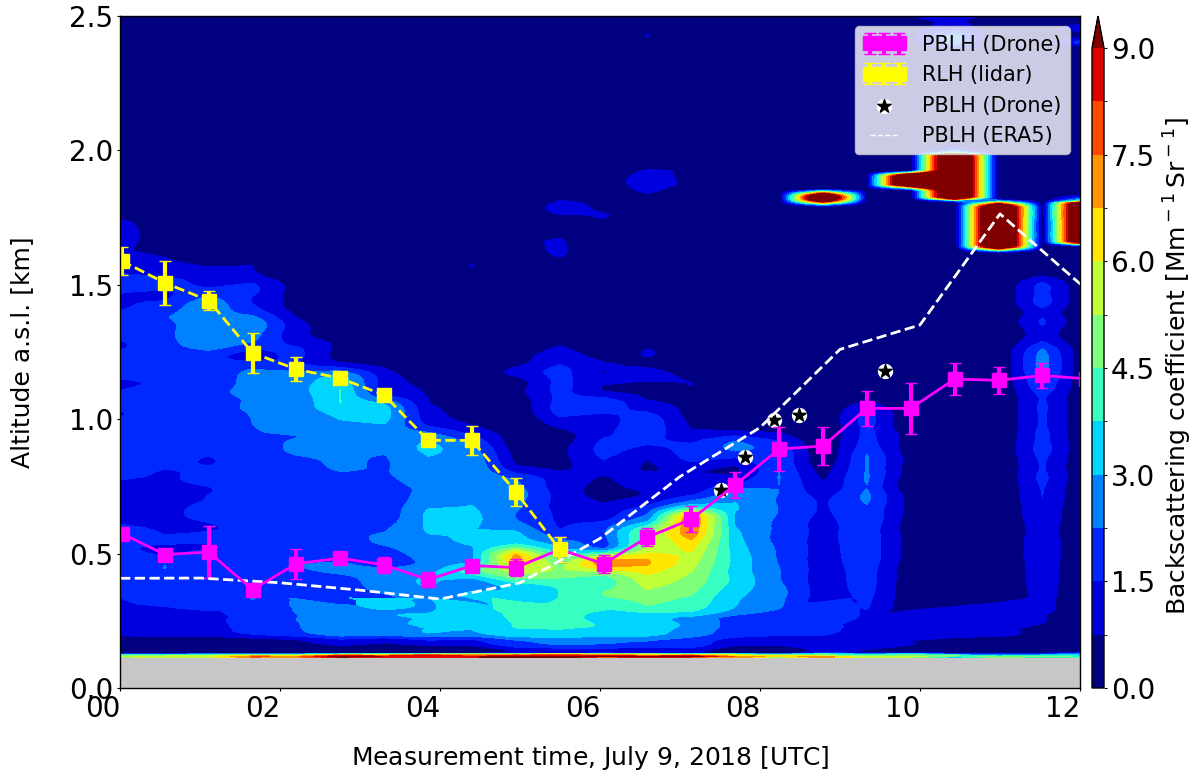
Figure 4 Time series of backscatter coefficients (contour), planetary boundary layer heights (PBLHs; pink squares) and residual layer heights (RLHs; yellow squares) retrieved from scanning lidar, as well as boundary layer heights obtained from UAV measurements (black star with a white circle surrounding it) and from the ERA5 dataset (dashed white line) measured by a UAV on 9 July 2018.

A comparison of the vertical profile of aerosols from lidar and UAV measurements was conducted using the following steps. First, we used the temperature and pressure measured by the UAV instead of an atmospheric model to calculate molecular backscatter coefficients, and these molecular backscatter profiles were used for lidar retrievals. Second, the backscatter coefficients at all observation angles were calculated using the Klett–Fernald method with reference values obtained from vertical profiles of the backscatter coefficients. Finally, Mie theory was used to calculate the aerosol backscatter coefficients based on size distributions measured by the UAV-borne OPC and the complex refractive index from a nearby Sun photometer. As there is no dryer before OPC-N3 sampling and no temperature difference between sampling tube and ambient environment, the effect of relative humidity on aerosol sampling was not considered. Figure 5 shows the backscatter coefficients retrieved from lidar measurements and from Mie calculations based on size distributions measured by the OPC on the UAV. In this experiment, the lidar performed zenith scans using elevation angles from 90 to 5° with steps of 5° during the UAV flights. Consequently, we retrieve the backscatter coefficients for each observation angle, and the average of these backscatter coefficients is shown as a thick red line to compare them with the UAV measurements. The average time is around 11 min for the lidar measurement from 08:14–08:25 UTC on 9 July 2018. This figure shows that the vertical distribution of the aerosol particles in the well-mixed boundary layer is reflected well in both lidar and OPC measurements. Furthermore, the backscatter coefficients from UAV retrievals (dashed green line in Fig. 5) show the same aerosol mixing height and the same order of backscatter coefficients as the lidar retrievals. The smaller backscatter coefficients calculated based on airborne OPC measurements may be related to an undercounting of the smaller particles, as we have seen for ground-based OPC measurements by the Fidas200 instrument. The size distributions were corrected by the counting efficiency curve introduced in Sect. 3.1. The backscatter coefficients from the corrected size distributions (dashed black line in Fig. 6) were consistent with the lidar-derived backscatter coefficients. Although Fidas200 is a different OPC sensor than OPC-N3, the same undercounting phenomenon was observed for both sensors. Please note that the particle size is averaged over 300 m, and the horizontal dashed lines represent these average altitude ranges. These vertical size distributions show that larger particles were detected only below 300 m above ground level.

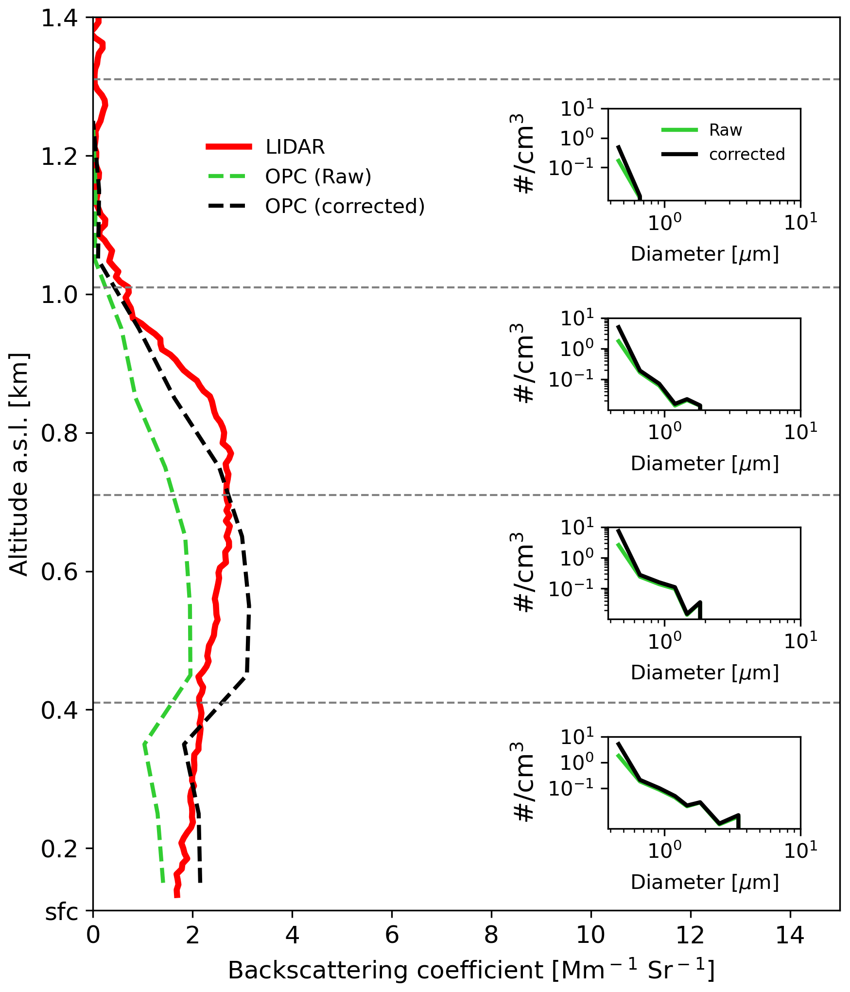
Figure 5 Vertical distribution of backscatter coefficients from lidar measurement (solid red line, averaged from 08:14–08:25 UTC), as well as backscatter coefficients derived from UAV-based measurements for raw size distributions (dashed green line) and corrected particle size distributions (dashed black line) (inserts on the right) on 9 July 2018. Note that “sfc” on the y axis indicates the ground surface level.

In total, 12 UAV flights were conducted on 9 and 12 July, as shown in Table 1 to compare with lidar retrievals. Figure 6 shows the correlation of backscatter coefficients retrieved from lidar measurement and from the Mie calculation based on aerosol size distributions measured by OPC-N3 on the UAV. The data from the lidar and UAV were averaged into 60 m vertical bins to reduce the noise of the OPC-N3 measurement. The colors of the scatter points indicated different UAV flights. This figure shows that the backscatter coefficients retrieved from lidar correlated on average with the backscatter coefficients calculated from the OPC with a slope of 0.789 ± 0.096 and a Pearson correlation coefficient of 0.234. This figure also shows that 75 % of the data points are within the grey shaded area, which indicates that these data are within a factor of 3. However, in contrast to the ground-level OPC measurements, a dedicated correction of the low-cost OPC data for potential sampling artifacts or undercounting was not possible. This figure also shows that the UAV measurements reflect the same aerosol mixing process within the boundary layer and the same order of magnitude of the backscatter coefficient. However, the backscatter coefficients retrieved from the UAV-borne OPC during certain UAV flights still show a relatively large deviation from the lidar retrievals. One reason for this variability is that the UAV cruising speed may affect the aerosol sampling by the OPC-N3. The samples were collected perpendicular to the flight direction into the OPC, so we can expect a size-dependent discrimination of larger particles. Compared to the Fidas200 OPC, as shown in Sect. 3.1, the OPC-N3 data show a significantly higher variability. This means that we must be careful with the quality and the operation of such in situ measurements, especially when no reference data like lidar are available.

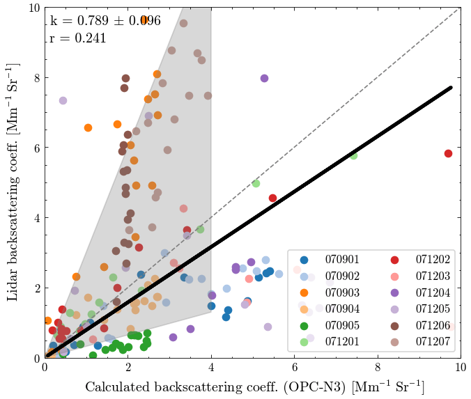
Figure 6 Correlation of backscatter coefficients retrieved from lidar measurement and modeled from Mie calculation based on aerosol size distribution measured by OPC-N3 on the UAV for all UAV flights on 9 and 12 July 2018. The different scatter point colors indicate different UAV flights. The thick black line is a linear fit to the data, and the thin dashed line is the 1 : 1 line.

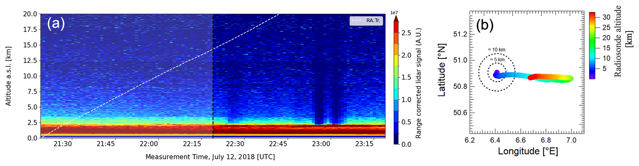
Figure 7 Time series of range-corrected lidar signal and radiosonde vertical trajectory (dashed white line) (a) and horizontal displacement of the balloon during this experiment (b) on 12 July 2018 at Jülich Research Center.

3.3 Comparison of lidar data with in situ measurements aboard a balloon

A balloon which carried the COBALD sensor to measure backscatter coefficients in situ was launched to an altitude of around 30 km on the night of 12 July 2018 to validate lidar retrievals. The lidar did vertically pointed measurements with an integration time of 60 s for each profile during the balloon launch. Figure 7a shows the range-corrected lidar signal for 2 h of continuous measurement and the vertical trajectory of the balloon. As shown in this figure, the lidar signal did not vary much in the first hour (the period was highlighted in this figure) while showing changes in the second half of the experiment. Hence, we selected the first hour to compare with balloon measurements. Figure 7b shows the horizontal trajectory of the radiosonde, with the color of the plot indicating the radiosonde altitude, and the circle indicating the distance from the lidar observation station. This figure shows that the horizontal displacement of the radiosonde is about 10 km when the radiosonde reached an altitude of 10 km, and this horizontal displacement may cause a difference in backscatter coefficients between lidar and COBALD. For the lidar analysis in this experiment, the backscatter coefficients were retrieved from elastic and Raman data with the vertical profiles of the molecular backscatter coefficient being calculated from temperature and pressure measured by the balloon. The COBALD data analysis follows the procedure proposed by Brunamonti et al. (2021). First, a wavelength extrapolation yielded the backscatter coefficient at a wavelength of 355 nm from COBALD measurement. The Ångström exponent (AE) used for this wavelength conversion is measured by COBALD at two wavelengths (455 and 940 nm) and extended to the wavelength of 355 nm. Second, as the FOV of the lidar and COBALD is different (the FOV of COBALD is 6°, whereas the FOV of lidar is 2.3 mrad), a FOV correction is necessary. The correction factors are calculated based on Mie theory and are shown in Fig. 2 in Brunamonti et al. (2021).

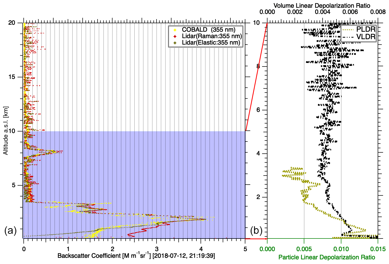
Figure 8 Backscatter coefficients measured by balloon-borne COBALD and lidar (a), as well as aerosol volume and particle depolarization ratio measured by lidar (b), on the night of 12 July 2018 at Jülich Research Center. (The integration time of the lidar data is 1 h from 21:19 to 22:19 UTC.)

Figure 8 shows the backscatter coefficients from COBALD and lidar measurement for a lidar integration time of 1 h. These two profiles of backscatter coefficients from lidar are retrieved from elastic and Raman channel data, respectively. The retrieval of backscatter coefficients from elastic channel data remained with a larger uncertainty due to the assumption of a lidar ratio in the Klett–Fernald method. Hence, it is more meaningful to compare backscatter coefficients from Raman data with those from COBALD measurements. In addition, the volume and particle depolarization ratios measured by lidar are shown on the right side of Fig. 8. The low depolarization ratios support our assumption that the particles are spherical and that we can use Mie calculations for the FOV correction. This figure shows a good agreement in the backscatter coefficients between lidar Raman data retrieval and COBALD measurement at an altitude above 2 km. However, there is a significant discrepancy at altitudes below 2 km.

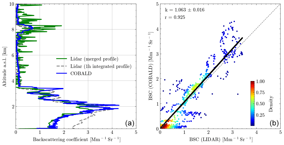
Figure 9 Profiles of backscatter coefficients from lidar for integration over 1 h (dashed grey line) and sliding 5 min merged backscatter coefficients (green line), as well as the vertical profile of an in situ backscatter coefficient measured by balloon-borne COBALD (blue line) on 12 July 2018 at the Jülich Research Center (a). The correlation between the lidar-merged backscatter coefficients and balloon-borne COBALD backscatter coefficients (b).

The discrepancy of the backscatter coefficients between lidar retrievals and COBALD measurements at lower altitudes is due to the temporal evolution of the aerosol particle concentrations in the boundary layer, as can be seen from vertical profiles of backscatter coefficients with a high temporal resolution in Fig. S5. This figure shows the profiles of backscatter coefficients retrieved from lidar Raman data with 5 min temporal resolution and backscatter coefficients measured by COBALD, as well as the vertical balloon trajectory. This figure shows a good agreement in the backscatter coefficients between COBALD measurement and lidar Raman data retrievals at the altitude of the balloon passing by. The backscatter values at the altitude of the balloon passing by are extracted, as shown as the red line in Fig. S5, to obtain merged Raman backscatter coefficients. The merged Raman backscatter coefficients and backscatter coefficients from COBALD measurements are shown on the left-hand side of Fig. 9, showing the very good agreement of backscatter coefficients from lidar and COBALD measurements at all altitudes. The correlation between lidar-merged Raman backscatter coefficients and COBALD backscatter coefficients is shown on the right-hand side of Fig. 9, which shows that these two backscatter coefficients are well correlated with a slope of 1.063 ± 0.016 and a Pearson correlation coefficient of 0.925. This consistency between lidar and COBALD sensor reflects a good data quality of both methods and proves that lidar can provide reliable and vertical profiles of aerosol particles with a high spatiotemporal resolution.

4 Conclusions

This paper presents results of aerosol spatiotemporal distribution and optical properties measured by a scanning aerosol lidar, a radiosonde with a backscatter sensor, an OPC-N3 on a UAV, and a comprehensive set of ground-level in situ measurements. Modern aerosol characterization methods including remote sensing and in situ methods helped us better understand the aerosol physical properties and build a bridge between remote sensing and these in situ methods. This paper focuses on the comparison of aerosol measurement between lidar retrievals and in situ measurements at ground level, in the troposphere, and in the stratosphere, thus validating lidar retrievals at all altitude levels.

The comparison of ground-level in situ extinction coefficients with lidar-derived ones shows that Fidas200 underestimated the particle number concentration by a factor of 2–10 at the diameter range between 0.25 and 0.5 µm, thus causing the total extinction calculated from this size distribution to be systematically lower than that from lidar retrievals by a factor of 4.70 ± 1.49. The extinction coefficient calculated from the Fidas200 aerosol size distribution corrected by the SMPS size distribution shows good agreement with the lidar-derived extinction coefficient, with a slope of 1.037 ± 0.015 and a Pearson correction coefficient of 0.878. The comparison also shows that the undercounting of aerosol particles between 0.25 and 0.5 µm is the main reason for the large discrepancy between lidar retrieval and ground-level in situ Fidas200 measurements. In addition, a comparison between lidar and UAV shows good agreement in the boundary layer height measurements, and both methods show a similar trend to the ERA5 boundary layer height evolution. The OPC-N3 aboard a UAV shows a similar aerosol vertical distribution and comparable backscatter coefficients to the lidar measurement. However, the backscatter coefficients calculated from OPC-N3 were unstable, and large uncertainties still remained for different flights, most likely due to the effect of UAV cruising on OPC-N3 sampling. Adapting the inlet design of the OPC may improve the data quality for future measurements. Finally, the backscatter from the balloon-borne COBALD measurement shows very good agreement with the backscatter retrieved from the lidar measurement if compared with 5 min resolution lidar data with a slope of 1.063 ± 0.016 and a Pearson correlation coefficient of 0.925. This consistency between the lidar and COBALD sensor validated our lidar retrievals and proves that lidar can provide reliable and high-resolution vertical profiles of aerosols. And this comparison highlights the complementary advantages of the lidar's continuous measurement capability and COBALD in situ two-wavelength data for characterizing aerosol particles from near-ground level up to the stratosphere. In conclusion, the retrievals from scanning aerosol lidar measurements show good agreement with in situ measurements at all altitude levels, and these lidar measurements can also be used as a reference for other low-cost in situ measurements.