Unchanged PM_2.5 levels over Europe during COVID-19 were buffered by ammonia

The coronavirus outbreak in 2020 had a devastating impact on human life, albeit a positive effect on the environment, reducing emissions of primary aerosols and trace gases and improving air quality. In this paper, we present inverse modelling estimates of ammonia emissions during the European lockdowns of 2020 based on satellite observations. Ammonia has a strong seasonal cycle and mainly originates from agriculture. We further show how changes in ammonia levels over Europe, in conjunction with decreases in traffic-related atmospheric constituents, modulated PM_2.5. The key result of this study is a −9.8 % decrease in ammonia emissions in the period of 15 March–30 April 2020 (lockdown period) compared to the same period in 2016–2019, attributed to restrictions related to the global pandemic. We further calculate the delay in the evolution of the ammonia emissions in 2020 before, during, and after lockdowns, using a sophisticated comparison of the evolution of ammonia emissions during the same time periods for the reference years (2016–2019). Our analysis demonstrates a clear delay in the evolution of ammonia emissions of −77 kt, which was mainly observed in the countries that imposed the strictest travel, social, and working measures. Despite the general drop in emissions during the first half of 2020 and the delay in the evolution of the emissions during the lockdown period, satellite and ground-based observations showed that the European levels of ammonia increased. On one hand, this was due to the reductions in SO₂ and NO_x (precursors of the atmospheric acids with which ammonia reacts) that caused less binding and thus less chemical removal of ammonia (smaller loss – higher lifetime). On the other hand, the majority of the emissions persisted because ammonia mainly originates from agriculture, a primary production sector that was influenced very little by the lockdown restrictions. Despite the projected drop in various atmospheric aerosols and trace gases, PM_2.5 levels stayed unchanged or even increased in Europe due to a number of reasons that were attributed to the complicated ${\mathrm{NH}}_{\mathrm{3}}-{\mathrm{H}}_{\mathrm{2}}{\mathrm{SO}}_{\mathrm{4}}-{\mathrm{HNO}}_{\mathrm{3}}$ system. Higher water vapour during the European lockdowns favoured more sulfate production from SO₂ and OH (gas phase) or O₃ (aqueous phase). Ammonia first reacted with sulfuric acid, also producing sulfate. Then, the continuously accumulating free ammonia reacted with nitric acid, shifting the equilibrium reaction towards particulate nitrate. In high-free-ammonia atmospheric conditions such as those in Europe during the 2020 lockdowns, a small reduction in NO_x levels drives faster oxidation toward nitrate and slower deposition of total inorganic nitrate, causing high secondary PM_2.5 levels.

1 Introduction

Ammonia (NH₃), the most abundant gas, has played a vital role in the evolution of the human population through the Haber–Bosch process (Chen et al., 2019). However, today it is recognized to have a significant negative influence on not only the environment (Stevens et al., 2010) but also the human population (Cohen et al., 2017; Pope and Dockery, 2006) and the climate (de Vries et al., 2011). As an alkaline molecule, ammonia regulates the pH of clouds, while its excessive atmospheric deposition and terrestrial runoff affect natural reservoirs, creating algae blooms and degrading water quality (Camargo and Alonso, 2006; Krupa, 2003). When emitted into the atmosphere, it reacts with the abundant sulfuric and nitric acids (Malm et al., 2004) to form sulfate, nitrate, and ammonium, contributing up to 50 % to the total aerosol mass (Anderson et al., 2003). The latter has implications for human health (Gu et al., 2014), as aerosols penetrate the human respiratory system and accumulate in the lungs (Pope et al., 2002), causing premature mortality (Lelieveld et al., 2015). Furthermore, through secondary aerosol formation (Pozzer et al., 2017), ammonia has a significant impact on (i) regional climate (Bellouin et al., 2011), causing visibility problems and contributing to the haze effect, and (ii) global climate directly by scattering incoming radiation (Henze et al., 2012) and indirectly as cloud condensation nuclei (Abbatt et al., 2006) that alter the Earth's radiative balance.

The largest portion of atmospheric ammonia originates from the synthesis of nitrogen fertilizers, which are in high demand for agriculture (Erisman et al., 2007). The expansion of intensive agriculture during the 20th century has increased atmospheric ammonia above natural levels (Erisman et al., 2008), while the projected growth of the global population will likely create larger nutritional needs that are expected to further increase ammonia emissions during the 21st century (Pai et al., 2021). Other sources of ammonia include emissions from livestock (Sutton et al., 2000), industry, ammonia-rich watersheds (Sørensen et al., 2003), traffic (Kean et al., 2009), sewage (Reche et al., 2012), humans (Sutton et al., 2000), biomass and domestic combustion (Sutton et al., 2008; Fowler et al., 2004), and volcanic eruptions (Sutton et al., 2008).

In past years, atmospheric ammonia observations were mostly limited to ground-based measurements from relatively sparse monitoring networks. This resulted in large emission uncertainties in regions that are poorly covered by measurements (Heald et al., 2012). Today, satellite products are capable of recording daily ammonia column concentrations, providing useful information on its atmospheric abundance. Recently, Van Damme et al. (2021) analysed Infrared Atmospheric Sounding Interferometer (IASI) retrievals and showed increased ammonia levels over most of Europe after 2015. Then, suddenly the COVID-19 outbreak came in 2020, creating a unique situation (Baekgaard et al., 2020) that affected all segments of life in a detrimental way (Chakraborty and Maity, 2020; Sohrabi et al., 2020). As a measure to inhibit further spread of the virus, authorities imposed strict social, travel, and working restrictions for months, which resulted in lower traffic-related emissions and improved air quality (Bauwens et al., 2020; Dutheil et al., 2020; Sicard et al., 2020). Illustrating the impact on emissions, Guevara et al. (2021) reported average emission reductions in Europe of 33 % for NO_x, 8 % for non-methane volatile organic compounds (NMVOCs), and 7 % for SO_x during the strictest lockdowns in 2020, while more than 85 % of the total reduction is attributed to road transport. CO₂ emissions also decreased by 11 % over Europe during the first lockdowns (Diffenbaugh et al., 2020), as did aerosols; notably, black carbon (BC) emissions dropped by 11 % (Evangeliou et al., 2021), and aerosol optical depth (AOD) decreased up to 20 % over central and northern Europe (Acharya et al., 2021).

While the COVID-19 lockdown impact on emissions of primary aerosols and trace gases has been studied extensively, how ammonia emissions were affected in Europe is unknown. This is very important and may have largely moderated the atmospheric levels of particulate matter (Giani et al., 2020; Guevara et al., 2021; Matthias et al., 2021) because of ammonia's contribution to secondary PM_2.5 (particulate matter) formation (Anderson et al., 2003). Here, we make use of satellite measurements of ammonia and a novel inversion algorithm to track how ammonia emissions changed before, during, and after the European lockdowns in 2020. We examine the reasons behind the estimated changes and validate the results against ground-based observations from the EMEP measurement network (https://emep.int/mscw/, last access: 26 August 2024; Fig. S1 in the Supplement). Finally, we calculate the resulting impact of ammonia changes on the formation of PM_2.5 during the European lockdowns using a chemistry–transport model (CTM) and try to interpret the mechanisms governing these changes.

2 Methods

2.1 Cross-track Infrared Sounder (CrIS) ammonia measurements

The CrIS sensor on board the NASA Suomi National Polar-orbiting Partnership provides atmospheric soundings at a high spectral resolution (0.625 cm⁻¹) (Shephard et al., 2015), resulting in improved vertical sensitivity for ammonia at the surface (Zavyalov et al., 2013). The CrIS fast physical algorithm (Shephard and Cady-Pereira, 2015) retrieves ammonia at 14 vertical levels using a physics-based optimal estimation retrieval, which also provides the vertical sensitivity (averaging kernels) and an estimate of the retrieval errors (error covariance matrices) for each measurement. Shephard et al. (2020) report a total column random measurement error of 10 %–15 %, with total random errors of ∼ 30 %. The individual profile random errors are 10 %–30 %, while total profile random errors increase above 60 % due to the limited vertical resolution (Shephard et al., 2020). Vertical sensitivity and error calculations are also important when using CrIS observations in satellite inverse modelling applications (Li et al., 2019; Cao et al., 2020), as a satellite observational operator can be generated in a robust manner (see next sections). The detection limit of CrIS measurements has been calculated down to 0.3–0.5 ppbv (Shephard et al., 2020), and the product has been validated extensively against ground-based observations (Dammers et al., 2017; Kharol et al., 2018), showing small differences and high correlations.

Daily CrIS ammonia satellite measurements (version 1.6.2) were gridded on a 0.5° × 0.5° grid covering all of Europe (25–75° N, 10° W–50° E,) from 1 January to 30 June 2020. Data were screened prior to use with a quality flag ≥ 4, as recommended in the CrIS documentation, and a cloud flag ≠ 1. The latter excludes retrievals that are performed under thin-cloud conditions, which are not as reliable as retrievals performed under cloud-free conditions (White et al., 2023). Gridding was chosen to limit the large number of observations (around 10 000 per day per vertical level for 2550 retrievals from January to June 2020), hence the need for a large number of source–receptor matrices (SRMs), which is computationally inefficient. Specifically, daytime and nighttime observations from CrIS were averaged in each 0.5° resolution grid cell daily from 1 January to 30 June 2020. This gridding method, although simple, gives more robust results than classic interpolation methods and presents small standard deviations of the gridded values (see Tichý et al., 2023). Sitwell et al. (2022) showed that the averaging kernels of CrIS ammonia are significant only for the lowest six levels (the upper eight have no influence on the satellite observations), and therefore we have considered these six vertical levels (∼ 1018–619 hPa).

2.2 Source–receptor matrix (SRM) calculations

SRMs were calculated for each 0.5° × 0.5° grid cell over Europe (25–75° N, 10° W–50° E,) using the Lagrangian particle dispersion model FLEXPART version 10.4 (Pisso et al., 2019) adapted to model ammonia. The model releases computational particles that are tracked backward in time using hourly ERA5 (Hersbach et al., 2020) assimilated meteorological analyses from the European Centre for Medium-Range Weather Forecasts (ECMWF), with 137 vertical layers and a horizontal resolution of 0.5° × 0.5°. FLEXPART simulates turbulence (Cassiani et al., 2015), unresolved mesoscale motions (Stohl et al., 2005), and convection (Forster et al., 2007). SRMs were calculated for 7 d backward in time, at temporal intervals that matched satellite measurements and at a spatial resolution of 0.5° × 0.5°. This 7 d backward tracking is sufficiently long to include almost all ammonia sources that contribute to surface concentrations at the receptors, given its typical atmospheric lifetime of about a day (Evangeliou et al., 2021; Van Damme et al., 2018).

The complicated heterogeneous chemistry of ammonia was modelled with the Eulerian model LMDz-OR-INCA, which couples the LMDz (Laboratoire de Météorologie Dynamique) general circulation model (GCM) (Hourdin et al., 2006) with the INCA (INteraction with Chemistry and Aerosols) model (Folberth et al., 2006; Hauglustaine et al., 2004) and with the land surface dynamical vegetation model ORCHIDEE (ORganizing Carbon and Hydrology In Dynamic Ecosystems) (Krinner et al., 2005). The model has a horizontal resolution of 2.5° × 1.3° and 39 hybrid vertical levels extending to the stratosphere. It accounts for large-scale advection of tracers (Hourdin and Armengaud, 1999), deep convection (Emanuel, 1991), while turbulent mixing in the planetary boundary layer (PBL) is based on a local second-order closure formalism. The model simulates atmospheric transport of natural and anthropogenic aerosols and accounts for emissions, transport (resolved and subgrid scale), and dry and wet (in-cloud/below-cloud scavenging) deposition of chemical species and aerosols interactively. LMDz-OR-INCA includes a full chemical scheme for the ammonia cycle and nitrate particle formation, as well as state-of-the-art ${\mathrm{CH}}_{\mathrm{4}}/{\mathrm{NO}}_x/\mathrm{CO}/\mathrm{non}-\mathrm{methanehydrocarbons}\left(\mathrm{NMHCs}\right)/{\mathrm{O}}_{\mathrm{3}}$ tropospheric photochemistry (Hauglustaine et al., 2014). The global transport of ammonia was simulated for 2020 with a month of spin-up by nudging the winds of the 3-hourly ERA5 data (Hersbach et al., 2020) with a relaxation time of 10 d (Hourdin et al., 2006).

For the calculation of ammonia's lifetime, LMDz-OR-INCA ran with traditional emissions for anthropogenic, biomass burning, and oceanic emission sources from ECLIPSEv5a (Evaluating the CLimate and Air Quality ImPacts of Short-livEd Pollutants), GFED4 (Global Fire Emission Dataset), and GEIA (Global Emissions InitiAtive) (hereafter called “EGG”) (Bouwman et al., 1997; Giglio et al., 2013; Klimont et al., 2017). FLEXPART uses the exponential mass removal for radioactive species based on the e-folding lifetime (Pisso et al., 2019), which gives the time needed to reduce the species mass to a $\mathrm{1}/e$ contribution. We calculated the e-folding lifetime (Kristiansen et al., 2016; Croft et al., 2014) of ammonia from LMDz-OR-INCA, assuming that the loss occurs as a result of all processes affecting ammonia (chemical reactions, deposition), with a minimum time step of 1800 s. Then we calculated the exponential loss of ammonia and the respective loss rate constant κ (s⁻¹). We point to Tichý et al. (2023) for more details on the methodology to avoid repetition.

Ammonia has complicated atmospheric chemistry and may react with sulfuric and nitric acid, producing sulfate and nitrate. However, under certain atmospheric conditions, the equilibrium reaction with nitric acid can be shifted to the left, producing free ammonia (Seinfeld and Pandis, 2000). Tichý et al. (2023) showed that production of free ammonia happened very rarely in continental Europe in the 2013–2020 period. Nevertheless, we have previously published a full validation of the CTM concentrations obtained vs. all the available ground-based measurements of ammonia globally (Tichý et al., 2023) from the EMEP network (https://emep.int/mscw/, last access: 26 August 2024) in Europe, EANET (East Asia acid deposition NETwork) in southeastern Asia (https://www.eanet.asia/, last access: 26 August 2024), and AMoN (Ammonia Monitoring Network in the US (AMoN-US) and the National Air Pollution Surveillance Program (NAPS) sites in Canada) in North America (http://nadp.slh.wisc.edu/data/AMoN/, last access: 26 August 2024).

2.3 Inverse modelling of ammonia emissions

The proposed inversion method is based on a comparison of the CrIS satellite observations and the model profile retrievals to estimate the spatiotemporal ammonia emissions. The comparison of remote-sensing observations such as CrIS with model (or in situ) profiles is not straightforward, as is the cases with ground-based observations. Here, we used the more rigorous approach of the “instrument operator” (see equation below) after interpolation of the model profile to the first six levels of the satellite product (Rodgers, 2000):

$$\begin{array}{}\text{(1)}& \ln \left(v^{\mathrm{ret}}\right)=\ln \left(v^{\mathrm{a}}\right)+\mathbf{A}\left(\ln \left(v^{\mathrm{true}}\right)-\ln \left(v^{\mathrm{a}}\right)\right),\end{array}$$

where v^ret is the retrieved profile concentration vector, v^a is the a priori profile concentration vector, v^true is the true profile concentration vector, and A is the averaging kernel matrix in logarithmic space (for each 0.5° × 0.5° resolution grid cell). In our inversion setup, we directly compared the retrieved v^ret and the observed satellite column concentration v^sat that is given by CrIS. In our case, v^true is equal to the modelled concentration v^mod calculated from the SRMs and a prior emission inventory. The argument for this approach is that v^ret is what the satellite would observe if v^mod were the true profile. This is a useful technique for evaluating whether the retrieval algorithm is performing as designed; i.e. is it unbiased, and whether the root-mean-square error (RMSE) calculated is within the expected variability. Further details about the algorithm and the setup can be found in Tichý et al. (2023).

The goal of the inversion is to iteratively update prior emissions, minimizing the distance between v^sat and v^ret by correcting the emission flux x in the term v^mod = srm^Flexx^a (srm^Flex denotes the FLEXPART SRMs) at each grid cell and in each of the six vertical levels that is important for CrIS (Sitwell et al., 2022):

$$\begin{array}{}\text{(2)}& \arg \underset{x^{\mathrm{a}}\to x}{min}{∥v^{\mathrm{sat}}-v^{\mathrm{ret}}∥}_{\mathrm{2}}^{\mathrm{2}}.\end{array}$$

The inverse problem is constructed for each spatial element of the computational domain. Inspired by the construction of the covariance matrix in Cao et al. (2020), we consider 4° surroundings (445 km), expressed by the index set 𝕊, for which the column concentrations are considered due to computational effectivity. Note that we observed low sensitivity of the resulting emission estimates to this choice. Then, we can formulate the inverse problem for each spatial element as

$$\begin{array}{}\text{(3)}& \left[{\mathit{v}}_{s_i}^{\mathrm{sat}};s_i\in \mathbb{S}\right]=\left[{\mathit{v}}_{s_i}^{\mathrm{ret}};s_i\in \mathbb{S}\right]q^{\mathbb{S}},\end{array}$$

where the left side of the equation is formed by the vector with aggregated CrIS observations, vectors ${\mathit{v}}_{s_i}^{\mathrm{ret}}$ form a block diagonal matrix, and q^𝕊 is an unknown vector with correction coefficients for each temporal element of the emission. The inverse problem in Eq. (3) was solved using the least squares with adaptive prior covariance (LS-APC) algorithm (Tichý et al., 2016). The algorithm is based on a Bayesian model, which assumes that all coefficients are positive and that the abrupt changes in their neighbouring values are less probable. It has been shown that this method is less sensitive to manual tuning of regularization parameters (see sensitivity tests in Tichý et al., 2020) than classical optimization procedures, which is crucial for such a large dataset where each spatial element represents a separate inverse problem.

A detailed description of the algorithm is given in Tichý et al. (2016). Here, we do not describe the algorithm again but explain a few modifications that were necessary for this study. By estimating the correction coefficients q^𝕊 for each grid cell of the spatial domain (25–75° N, 10° W–50° E), we can propagate the coefficients through Eq. (2) to update a priori emissions x^a in the model concentration term v^mod. We follow Li et al. (2019) and Cao et al. (2020) to bound the ratio between the prior and the posterior emissions. The lower and upper bounds of this ratio are set to 0.01 and 100, respectively, to omit the unrealistically low or high emissions. We consider these bounds large enough to allow new emission sources not present in the prior emissions to be exposed.

We evaluate the performance of the inversion using three a priori emission datasets: (i) one based on the Van Damme et al. (2018) calculations (hereafter “VD”, corresponding to VDgrlf emissions from Evangeliou et al., 2021); (ii) the ECLIPSEv6b inventory (Zbigniew Klimont, personal communication, 2022; Klimont et al., 2017) combined with biomass burning emissions from GFEDv4 (Giglio et al., 2013) as the most recent one (denoted “EC6G4”); and (iii) the average of four emission inventories for ammonia except for the two mentioned before, “EGG” (see previous section) and “NE” calculated from IASI (Infrared Atmospheric Sounding Interferometer) observations (Evangeliou et al., 2021) (denoted “avgEENV”). To account for the spatiotemporal impact of the lockdown on the European emissions, we corrected prior emission inventories of ammonia (only the bottom-up EGG and EC6G4, the top-down ones are based on satellite measurements where possible changes due to COVID-19 have been captured) for 2020 using the adjustment factors (AFs) adopted from Doumbia et al. (2021). The same was done for SO₂ and NO_x (precursors of sulfuric and nitric acid in the atmosphere) in EGG, which was used to calculate ammonia's loss rates using the LMDz-OR-INCA model (see Sect. 2.2). This dataset provides, for the January–August 2020 period, gridded AFs at a 0.1° × 0.1° resolution on a daily resolution for the transportation (road, air, and ship traffic), power generation, industry, and residential sectors. The quantification of AFs is based on activity data collected from different databases and previously published studies. These emission AFs have been applied to the CAMS global inventory, and the changes in emissions of the main pollutants have been assessed for different regions of the world in the first 6 months of 2020 (Doumbia et al., 2021).

Figure 1 shows the comparison of prior and posterior concentrations vs. independent observations (observations that were not used in the inversion algorithm) from the EMEP network (https://emep.int/mscw/, last access: 26 August 2024, Fig. S1) for January–July 2020. Note that prior concentrations of ammonia result from coupling the FLEXPART SRMs with prior emissions (from VD, ECLIPSEv6b, and avgEENV), while posterior concentrations come from coupling the SRMs with the calculated posterior emissions. In Fig. 1, it is evident that the most accurate reconstruction of surface concentrations with respect to the EMEP observations was obtained using avgEENV as the a priori information, and therefore the results presented hereafter are based on this setup. We performed inversions for the first half of 2020 to assess the effect of lockdown measures on ammonia emissions, as well as the situation after lockdown measures were taken away (rebound period). To have a more generic view, we also performed inverse modelling calculations for the first half of each year between 2016 and 2019 (reference period). Then, we assess the impact of ammonia changes on aerosol formation (PM_2.5) by feeding the posterior emissions to the LMDz-OR-INCA model and calculating the production of PM_2.5.

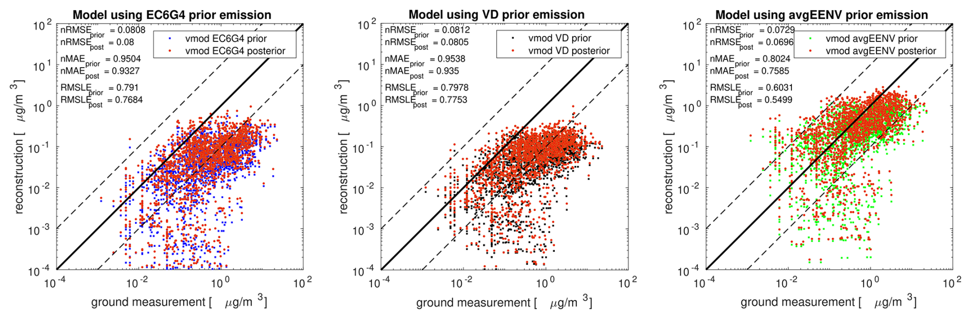
Figure 1 Scatterplots of prior and posterior concentrations vs. independent observations (observations that were not included in the inversion algorithm) from the EMEP network (https://emep.int/mscw/, last access: 26 August 2024, Fig. S1) from January to July 2020. Three statistical measures (nRMSE, nMAE, and RMSLE) were used to assess the performance of each inversion using three different prior emission inventories for ammonia (EC6G4, VD, and avgEENV).

2.4 Statistical tests

To evaluate the comparisons between modelled and observed concentrations of ammonia, we used the root-mean-squared logarithmic error (RMSLE) defined as follows:

$$\begin{array}{}\text{(4)}& \begin{array}{rl}& \text{RMSE}=\sqrt{{\sum }_{i=\mathrm{1}}^N{\displaystyle \frac{{\left(C_{\mathrm{m}}-C_{\mathrm{o}}\right)}^{\mathrm{2}}}{N}}}\text{and}\\ & \text{RMSLE}=\sqrt{{\displaystyle \frac{\mathrm{1}}{N}}{\sum }_{i=\mathrm{1}}^N{\left(\log C_{\mathrm{m}}-\log C_{\mathrm{o}}\right)}^{\mathrm{2}}},\end{array}\end{array}$$

where C_m and C_o are the modelled and measured ammonia concentrations, and N is the total number of observations. The commonly used Pearson squared correlation coefficient (r) was also used as a measure of linear correlation between two sets of data, defined as

$$\begin{array}{}\text{(5)}& r={\displaystyle \frac{\sum \left(C_{\mathrm{m}}-\stackrel{\mathrm{‾}}{C_{\mathrm{m}}}\right)\left(C_{\mathrm{o}}-\stackrel{\mathrm{‾}}{C_{\mathrm{o}}}\right)}{\sqrt{{\left(C_{\mathrm{m}}-\stackrel{\mathrm{‾}}{C_{\mathrm{m}}}\right)}^{\mathrm{2}}{\left(C_{\mathrm{o}}-\stackrel{\mathrm{‾}}{C_{\mathrm{o}}}\right)}^{\mathrm{2}}}}},\end{array}$$

where the distance of modelled and measured ammonia concentrations from the mean ($\stackrel{\mathrm{‾}}{C_{\mathrm{m}}}$ and $\stackrel{\mathrm{‾}}{C_{\mathrm{o}}}$) is computed. Finally, the standard deviation was adopted as a measure of the dispersion of modelled ammonia from the observations, which is the true value:

$$\begin{array}{}\text{(6)}& \mathit{\sigma }=\sqrt{{\displaystyle \frac{{\left(C_{\mathrm{m}}-C_{\mathrm{o}}\right)}^{\mathrm{2}}}{N}}}.\end{array}$$

The mean fractional bias (MFB) was selected as a symmetric performance indicator that gives equal weight to under- or overestimated concentrations (minimum to maximum values range from −200 % to 200 %). It was used in the independent validation (validation against measurements that were excluded from the inversion; see Sect. 3.3) of the posterior concentrations of ammonia during the European lockdowns of 2020 and is defined as

$$\begin{array}{}\text{(7)}& \text{MFB}={\displaystyle \frac{\mathrm{1}}{N}}{\displaystyle \frac{{\sum }_{i=\mathrm{1}}^N\left(C_{\mathrm{m}}-C_{\mathrm{o}}\right)}{{\sum }_{i=\mathrm{1}}^N\left(\frac{C_{\mathrm{m}}+C_{\mathrm{o}}}{\mathrm{2}}\right)}}.\end{array}$$

For the same reason, the mean absolute error was computed and normalized (nMAE) over the average of all the actual values (observations here), which is a widely used simple measure of error:

$$\begin{array}{}\text{(8)}& \text{MAE}={\displaystyle \frac{{\sum }_{i=\mathrm{1}}^N\left|C_{\mathrm{m}}-C_{\mathrm{o}}\right|}{{\sum }_{i=\mathrm{1}}^N{C}_{\mathrm{o}}}}.\end{array}$$

3 Results

3.1 Ammonia emission changes due to COVID-19 restrictions over Europe

The reason behind the three priors used in the inversion (EGG, EC6G4, and avgEENV) of ammonia is three-fold: (i) they are based on the most recent estimates, (ii) they are present at different spatial distributions, and (iii) they were derived using different methodologies. More specifically, EC6G4 is based on the emission model GAINS (Klimont et al., 2017), while VD uses satellite observations combined with a box model (Evangeliou et al., 2021). As mentioned in the previous section, we saw that the most accurate representation of surface model concentrations was achieved using the avgEENV a priori, which forces posterior concentrations closer to the 1 : 1 line, and the statistics obtained are significantly better than using other priors (Fig. 1). Therefore, the results presented below have all been obtained using avgEENV as the prior emission dataset, keeping results using the other two priors in the Supplement.

The total prior emissions of ammonia over Europe for the inversion period (January–June), the posterior emissions for the years 2016–2019, and the posterior emissions during the lockdown year 2020 (January–June) are plotted in Fig. 2 (the results from inversions using EC6G4 and VD prior emissions are illustrated in Figs. S2 and S3). The total prior ammonia emitted between January and June in Europe was equal to 1061 kt (Fig. 2a). To check whether the changes calculated in 2020 were due to meteorology and to avoid misinterpretation of our findings, inverse calculations of ammonia were performed for the reference years of 2016–2019 (January–June) using the observations from CrIS and exactly the same set-up as the one described in Sect. 2 (Methods). The total posterior emissions of ammonia over Europe for the reference period (2016–2019) were estimated to be 1665 ± 330 kt (4-year mean ± SD), or 57 % higher than the prior (Fig. 2b). Finally, for January–June 2020, the emission estimates derived were equal to 1568 ± 732 kt (posterior ± uncertainty) (Fig. 2c). This is 48 % higher than the prior and 6 % lower than the posterior emissions of January–June 2016–2019.

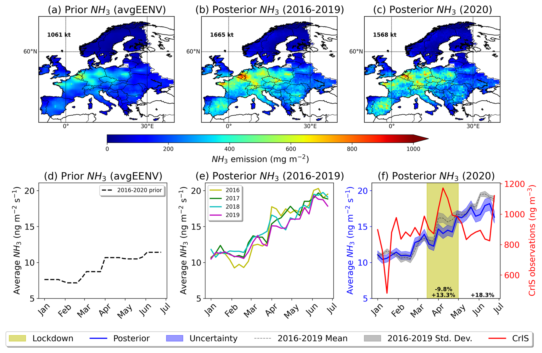
Figure 2 (a) Total a priori emissions of ammonia over Europe for the inversion period (January–June). The emissions correspond to the avgEENV prior, and the total emitted amount is equal to 1061 kt. (b) Total a posteriori emissions of ammonia over Europe for the inversion period (January–June) during the reference period 2016–2019 (using the avgEENV prior) that amount to 1665 kt. (c) Total posterior emissions of ammonia over Europe for January–June 2020 (1568 kt) using avgEENV as the prior. (d) Time series of weekly average prior emissions of ammonia over Europe (January to June 2020) from the avgEENV prior. (e) Time series of weekly average posterior emissions of ammonia over Europe for the reference years of 2016–2019 (January to June) (yellow, green, cyan, and magenta colours). (f) Time series of weekly average posterior emissions of ammonia with the associated uncertainties over Europe in 2020. Results from inversions using the avgEENV prior are plotted together with the CrIS observations averaged over Europe (red line) and the mean ammonia emissions with the calculated standard deviations for the reference period (2016–2019). The top value in the yellow highlighted area (−9.8 %) shows the percentage change in ammonia emissions during the 2020 lockdown compared to the same period in the reference years, whereas the two values just above the x axis in the yellow highlighted area show the corresponding changes in ammonia emissions (i) during the 2020 lockdown compared to the period before lockdown (+13.3 %) and (ii) after lockdown finished compared to the lockdown period (+18.3 %), known as rebound period.

The weekly average evolution of prior and posterior emissions of ammonia over Europe (January to June) for 2016–2019 shows a similar pattern, with small year-to-year variability (Fig. 2d, e) and similar temperatures (Fig. S4), thus there is no significant impact from the prevailing meteorology that would justify the change in emissions due to volatilization. The weekly posterior ammonia emissions over Europe changed during the lockdown period (2020) compared to the reference years (Fig. 2f). Satellites and national monitoring measurements of ammonia show that emissions peak in spring (March) and late summer in Europe (Van Damme et al., 2022), corresponding to the two main fertilization periods (Paulot et al., 2014). Ammonia abundances are, however, high throughout the entire spring–summer period due to agriculture associated with rising temperature (Sutton et al., 2013). Ammonia posterior emissions in the period of 15 March–30 April 2020 (European lockdown) declined by −9.8 % compared to the same period over the previous 4 years (2016–2019; Fig. 2f). Although the posterior emissions obtained for the reference period (dashed grey line and shading) are very similar to those from 2020 (solid blue line and shade in Fig. 2f), emissions during the lockdown period in 2020 dropped substantially, outside of the deviation in the emissions in the reference period (Fig. 2f).

3.2 Uncertainty in the posterior emissions

As described in Sect. 2.3 in more detail, we considered the 4° surroundings of each spatial element in our inversion domain from which the CrIS observations were used in the inverse problem. This means that 45 spatial elements in CrIS space were used, each with six vertical levels, for each of the 26 temporal emission elements. To calculate the associated uncertainty in the posterior estimates, we tested two sources of uncertainty: (i) how different surroundings for each spatial element affect posterior emissions of ammonia and (ii) how the use of different prior emissions affects posterior ammonia. We organized a series of sensitivity tests using the surroundings that are 2, 3, and 4° from each grid cell. This selection is realistic, as it was shown previously in Cao et al. (2020) for the construction of a prior emission error covariance matrix. For the second source of uncertainty, we performed the same inversion using not only EC6G4 and VD priors but also results from two more datasets for ammonia (in total four), which have 10-times-higher emissions, namely EGG and NE (see Sect. 2.3).

The absolute uncertainties calculated are depicted in Fig. 3a–c together with the relative uncertainty (Fig. 3d) with respect to the posterior emissions of ammonia (posterior ammonia is shown in Fig. 2c). The first source of uncertainty (different surroundings) affects the resulting posterior emissions of ammonia slightly (Fig. 3a), causing an average relative uncertainty below 4 % in the European emissions. The second source of uncertainty (use of different priors) causes a much larger bias, as shown in Fig. 3b (average relative uncertainty of 35 %). The reason for this is obviously the large variation in the EGG (Bouwman et al., 1997; Giglio et al., 2013; Klimont et al., 2017) and NE (Evangeliou et al., 2021) prior datasets that have total emissions in the first half of 2020 of 63.5 and 53.3 Tg, respectively, in contrast to only 6.2 and 5.7 Tg for EC6G4 and VD. Hence, the results presented here are sensitive to the use of the prior emission dataset. The modelled concentrations (that replace the hypothetical true column concentration in Eq. 1) are calculated by the SRMs and the prior emission and, therefore, play a key role in the comparison of the CrIS value (v^sat) and retrieved value (v^ret) (see Eq. 2). Also, the modelled concentrations depend on the natural logarithm weighted by the averaging kernel in logarithmic space. The linearization of this operator, as suggested by Sitwell et al. (2022), may reduce the dependency on the prior emission term; however, this is beyond the scope of this study. Overall, the propagated (absolute and relative) uncertainties in the posterior emissions are shown in Fig. 3c and d and are equal to 66 % over Europe on average (Fig. 3). This shows that our calculations are, on the one hand, robust but, on the other, are dependent on the use of a priori information.

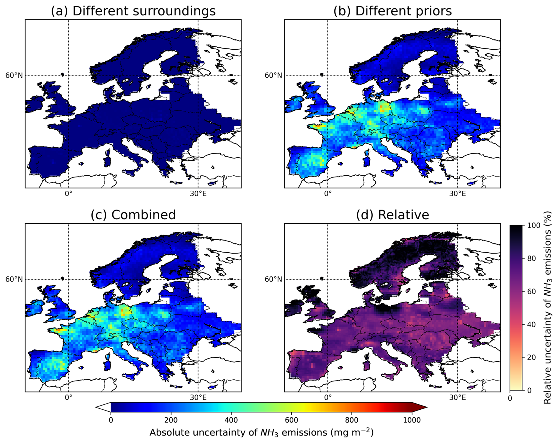
Figure 3 (a) Absolute uncertainty from the use of different surrounding grid areas for each spatial element of our inversion domain in the sensitivity tests; 2 to 4° grid cells were considered, resulting in a mean relative uncertainty of 4 %. (b) Absolute uncertainty from the use of four different prior emission estimates, namely EC6G4, VD, EGG, and NE (see Sect. 2.3). Here, a much larger uncertainty was calculated due to the use of 10-fold-higher prior emission datasets. (c) Propagated absolute uncertainty from the different sensitivity tests and (d) relative uncertainty with respect to the posterior emissions (Fig. 2c). The average uncertainty in the inversion domain for the first half of 2020 was estimated to be 66 %.

3.3 Validation of posterior ammonia vs. independent measurements

The optimized emissions of ammonia must be validated against independent observations because the inversion algorithm has been designed to reduce the model–observation mismatches. Here, the reduction in the posterior concentration differences compared to the observations from CrIS is determined by the weighting that is given to the observations, and, hence, such a comparison depends on this weighting (dependent observations). Therefore, the ideal comparison of any posterior emission resulting from top-down methods would be vs. measurements that were not included in the inversion algorithm (independent observations). Here, we used ground-based observations of ammonia from all EMEP sites (https://emep.int/mscw/, last access: 26 August 2024) for the period of our study as an independent dataset for validation. All stations are illustrated in Fig. S1.

As we mentioned in Sect. 2.3, we evaluated the efficiency of the inversion and the most effective a priori dataset for our purpose by assessing the match between the calculated posterior concentrations and all available observations from EMEP (N = 3957) for the study period (Fig. 1). More specifically, after it became evident that the most accurate results were obtained with avgEENV as the prior (relationship closer to unity compared to measured ammonia), we saw an immediate improvement in the statistical tests used (nRMSE, nMAE, and RMSLE) when using the posterior emissions to model ammonia in FLEXPART during the first half of 2020 (Fig. 1, right panel). nMAE decreased from 0.80 using the prior emissions to 0.76 using the posterior ones; accordingly, nRMSE of the posterior concentrations dropped to 0.073 compared to −0.069 using the prior emissions, while the RMSLE decreased from 0.60 using prior emissions to 0.55 using the optimized a posteriori emissions. To get a better insight into how modelled concentrations improved vs. the ammonia observations, eight random EMEP stations were selected to show time series of prior and posterior concentrations in the first half of 2020 (Fig. S5). Although large peaks were not reproduced, all statistics were improved when using the posterior emissions of ammonia.

3.4 Country-level changes due to COVID-19 restrictions

To document the emission changes in ammonia over the different European countries before, during, and after the 2020 lockdowns, we report the weekly evolution of the emissions for 16 countries individually (Fig. 4). Specifically, weekly emissions were averaged for each country based on the country definitions that are shown in Fig. S6 using the avgEENV prior.

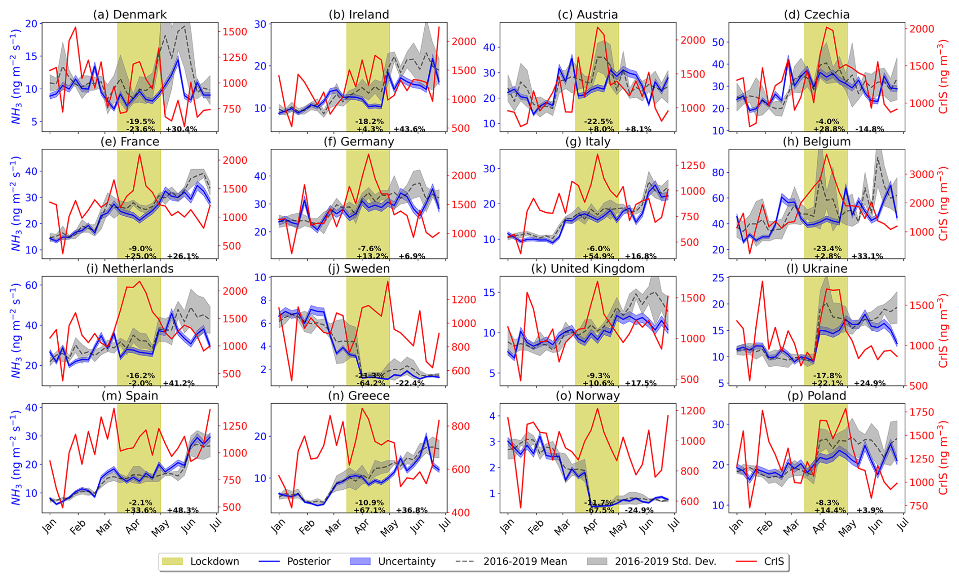
Figure 4 Time series of weekly average posterior emissions of ammonia (blue lines) with the calculated uncertainties (blue shading) in different European countries in 2020, resulting from inversions using prior information from avgEENV plotted together with the CrIS observations (red lines) and mean emissions (dashed lines) with the calculated standard deviations (grey shading) for the reference period (2016–2019). The top values in the highlighted areas show the change in ammonia emissions during the 2020 lockdowns (15 March–30 April) compared to the same period the in the years before (2016–2019), whereas the two values just above the x axis in the yellow highlighted area show the changes in ammonia emissions during the 2020 lockdown compared to (i) the period before the lockdown and (ii) the period after lockdown finished vs. the lockdown period (rebound period).

Most countries show that ammonia emissions declined or at least were less affected by the 2020 lockdowns compared to the same period during the reference years (2016–2019). Countries with substantial decreases in 2020 lockdown emissions were the Netherlands (−16 %) and Belgium (−23 %), both countries with important agricultural activity, as well as Denmark (−20 %), Ireland (−18 %), and Ukraine (−18 %). Smaller changes were recorded in Spain (−2.1 %), Czechia (−4.0 %), and Italy (−6.0 %) despite the intensive lockdown measures. This shows in practice that agricultural activity is not significantly affected, even in periods of extraordinary austerity, as it is the last remaining primary production sector necessary for human life.

We note that the largest emissions of ammonia in European countries were seen around March–April (weeks 8–16) and in summer. These coincide with the fertilization periods mentioned previously (Paulot et al., 2014) that control the seasonality of ammonia's emissions. In most European countries, the time of the year when fertilizers can be applied is tightly regulated (Ge et al., 2020). For instance, in the Netherlands and Belgium, the largest ammonia contributing region in Europe, application of nitrogen fertilizer is only allowed from February to mid-September. This produces two peak periods, in March and in late May (Fig. 4). Manure application also follows stringent regulations and is only allowed in the same periods depending on the type of manure (slurry or solid) and the type of land (grassland or arable land) (Van Damme et al., 2022).

To understand and position where the ammonia emissions changed during the European lockdowns of 2020, we plot the difference in the posterior emissions of ammonia during the lockdown period (15 March–30 April) for the same period in Fig. 5a. We calculate higher emissions of ammonia (+115 kt) during the lockdown compared to the prior emissions. Note that inversion algorithms aim to reduce the mismatches between modelled concentrations and observations (in our case, from CrIS satellite measurements) by correcting emissions. This means that different posterior emissions are most likely due to errors in the prior emissions and do not indicate any impact from the restriction measures.

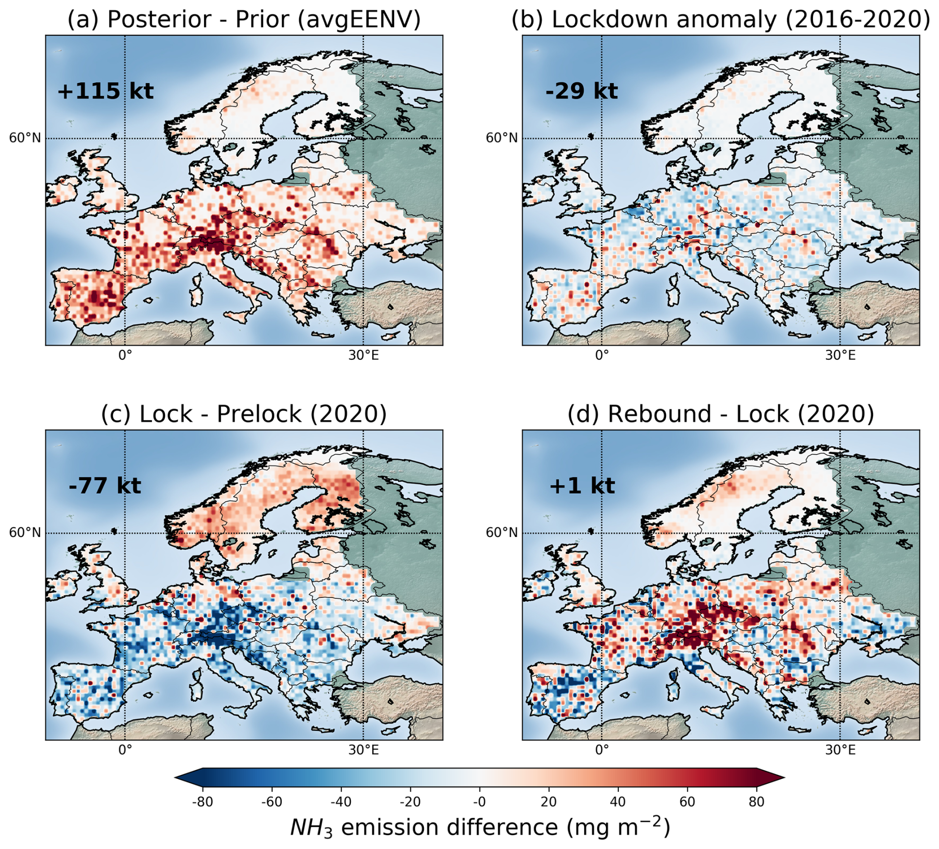
Figure 5 (a) The difference between posterior and prior emissions of ammonia during the European lockdowns of 2020 (15 March–30 April) using the avgEENV emissions as the prior. (b) Emission anomaly relative to the 2020 lockdowns from the 2016–2020 period (15 March–30 April). The difference in posterior ammonia (c) during the 2020 lockdowns (15 March–30 April; lock) vs. the period before (1 January–14 March) and (d) after the 2020 lockdowns (1 May–31 June; rebound) vs. the period during the 2020 lockdowns (15 March–30 April; Lock) compared to the reference years (2016–2019).

Therefore, we demonstrate the impact of the COVID-19 lockdowns over Europe in 2020 by calculating the emission anomaly for the lockdown period from 2016–2020 (the same period as the 2020 lockdowns, namely 15 March–30 April) in Fig. 5b. Emissions during the 2020 lockdowns dropped by −29 kt with respect to the same period in 2016–2020, showing the impact of the COVID-19 restrictions. The maximum decreases were seen in the Netherlands and Belgium, both countries with high emissions (Fig. 5b) that also suffered heavily from the COVID-19 outbreak (Anderson et al., 2020) and enforced strict lockdown measures. Other areas where significant changes were calculated were northern Italy, Switzerland, and Austria, while Scandinavian countries were not affected. This agrees well with the state of the epidemic in these countries in spring 2020. While Italy (specifically the northern region) was the first country outside China to suffer high mortality rates and, thus, dramatic social restrictions in spring 2020, Norway, Sweden, Denmark, and Finland showed total infected cases far below 1 % per capita, mostly suffering higher rates later in 2020 (Gordon et al., 2021).

As mentioned previously, ammonia emissions increase in spring (March) and late-summer in Europe (Van Damme et al., 2022; Paulot et al., 2014). Therefore, calculating the difference in the emissions during the lockdown vs. the period before or after is practically meaningless and cannot show the lockdown's impact since agricultural activity was only slightly affected in 2020. For this reason, we quantify the delay in the evolution of the 2020 emissions by calculating emission differences in the lockdowns vs. the period before (lock–prelock) for the lockdown year 2020 and emission differences (lock–prelock) for the reference years (2016–2019). Then, we plot their spatial differences in Fig. 5c. Accordingly, we do the same calculation for differences in the rebound period (the period after the restrictions were relaxed) vs. the lockdown period (rebound–lock) in 2020 and compare them to the same period for the reference years 2016–2019 (Fig. 5d). We observe a clear delay in the evolution of ammonia emissions of −77 kt in 2020 (Fig. 5c), while only Scandinavian countries show positive changes. Hotspots of negative evolution were seen in central Europe, mainly in the trio of northern Italy, Switzerland, and Austria, for the reasons discussed in the previous paragraph. In Poland, social measures affected the daily lives of citizens significantly (Szczepańska and Pietrzyka, 2021) and might be the reason for the decreased evolution of ammonia emissions (Fig. 5c). After the measures were relaxed, the evolution of the emissions rebounded slightly with respect to the reference period (2016–2019), as shown in Fig. 5d. The changes in ammonia during the rebound period were concentrated in countries that were affected most severely by the lockdown restrictions, namely northern Italy, Switzerland, Austria, and Poland. The same has been reported elsewhere for several other pollutant emissions (Davis et al., 2022; Jackson et al., 2022).

4 Discussion

4.1 Rising ammonia concentrations during the European lockdowns

One issue that has been overlooked is the concentrations of ammonia before, during, and after the 2020 lockdowns in Europe. Despite the delay in the emissions during the lockdown period in 2020 (Sect. 3.4), satellite ammonia from CrIS showed an increase during the lockdowns and declined after the restrictions were relaxed in almost all European countries (Fig. 4). This decline was reported in several studies analysing ground-based measurements. For example, Lovarelli et al. (2021) concluded that contrary to other air pollutants, ammonia was not reduced when the COVID-19 restrictions were introduced in north Italy. They further reported that urban and rural ammonia was the highest compared to previous years during the same months that the strictest lockdowns occurred (i.e. spring 2020). Rennie et al. (2020) reported a slight decrease in ammonia in the UK, while Xu et al. (2022) observed increased ambient ammonia during the lockdowns in China. Accordingly, Viatte et al. (2021) found enhanced ammonia during lockdown in Paris. Finally, in a recent study, Kuttippurath et al. (2023) reported an increase in ammonia during lockdowns almost everywhere, with maxima in western Europe, eastern China, the Indian subcontinent, and the eastern USA. Since atmospheric ammonia has been increasing globally due to various anthropogenic activities, the European lockdowns in 2020 offer a unique opportunity to expose ammonia's sources and address the importance of secondary PM_2.5 formation.

Figure 6a depicts the modelled atmospheric lifetime of ammonia and its dependence on the calculated loss rates over Europe for the first half of 2020. Ammonia is a particularly interesting substance due to its ability to react with atmospheric sulfuric and nitric acids, producing secondary aerosols. However, the reaction with sulfuric acid is more prevalent due to several factors. For instance, sulfuric acid is a stronger acid than nitric acid, leading to more efficient reactions with ammonia (higher reaction rate constant for ammonia with sulfuric than with nitric acid and thus faster formation of ammonium sulfate) (Behera and Sharma, 2012). Furthermore, ammonium sulfate (the final product of ammonia reaction with sulfuric acid) is less volatile and more thermodynamically stable than ammonium nitrate (the product of the reaction with nitric acid), favouring the formation and persistence of ammonium sulfate particles in the atmosphere (Walters et al., 2019). Finally, sulfuric acid forms more stable clusters with ammonia, even in the presence of nitric acid (Liu et al., 2018). Results from laboratory and field studies have confirmed that ammonia actually promotes the nucleation of sulfuric acid in the atmosphere (Weber et al., 1999; Schobesberger et al., 2015). The CLOUD (Cosmics Leaving Outdoor Droplets) experiment has also highlighted the fact that ammonia preferentially reacts with sulfuric acid in the atmosphere due to its strong acidity, ability to drive stable aerosol formation, and significant nucleation enhancement effects (Kirkby et al., 2016; Wang et al., 2022). Nitric acid plays a secondary role, primarily forming ammonium nitrate once sulfuric acid has reacted, but its contribution is limited by its volatility.

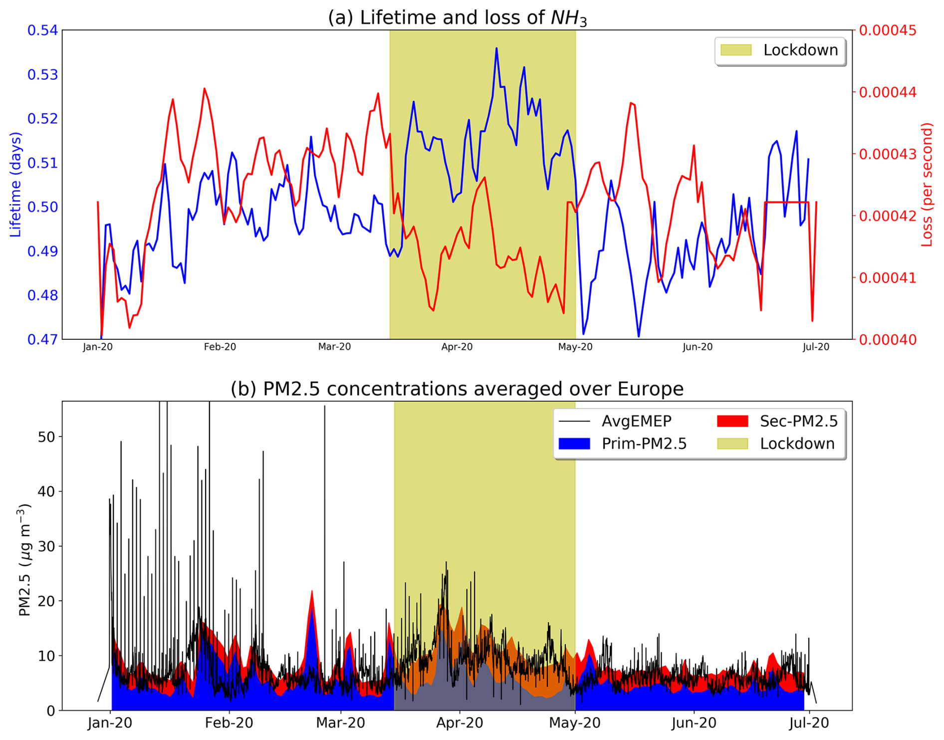
Figure 6 (a) Modelled lifetime (blue) and loss rates (red) of atmospheric ammonia averaged over Europe for January–June 2020. The lockdown period (15 March–30 April) is shaded in yellow. Right after COVID-19 restrictions were applied, loss rates of ammonia (shown in red) were disturbed due to reported decreases in SO₂ and NO_x (Guevara et al., 2021; Doumbia et al., 2021), the precursors of sulfuric and nitric acids (with which ammonia reacts to form PM_2.5) and the constant accumulation of atmospheric ammonia. This had an effect on the lifetime of ammonia (plotted in blue), which started increasing in Europe, leading to further accumulation of ammonia. (b) Observations of PM_2.5 from the EMEP stations (78 stations) plotted against modelled PM_2.5 concentrations, both averaged over Europe, from primary sources and secondary formation. It is evident that right after lockdown (yellow highlight), secondary PM_2.5 formation maintained high concentrations across Europe.

During the lockdown period in Europe, transport and industrial activities mostly stopped, and consequently the related emissions also decreased. This had an immediate effect on SO₂ and NO_x (Guevara et al., 2021; Doumbia et al., 2021). Reductions in SO₂ and NO_x caused less production of atmospheric sulfuric and nitric acids. The latter had a rapid two-fold effect on the lifetime of ammonia: (i) fewer available atmospheric acids needed less ammonia to create sulfate (mainly) and nitrate aerosols (secondarily), and therefore the loss rates declined (Fig. 6a), leading to accumulation of ammonia in its free form, and (ii) ammonia originates mainly from agriculture and livestock, and these activities were only slightly affected during the European lockdowns, increasing the associated emissions (see Fig. 2, although with a lower trend than previous years, as discussed in Sect. 3.4). The rising levels of ammonia during the COVID-19 lockdowns in Europe have been confirmed by the CrIS observations (Figs. 2 and 3) and have been also reported elsewhere (Kuttippurath et al., 2023; Viatte et al., 2021; Xu et al., 2022; Lovarelli et al., 2021).

4.2 Disturbance in the secondary formation of PM_2.5

The response of PM_2.5 mass concentrations to the restriction measures suggests a relationship that is more complex than expected and beyond road traffic intensity, at least for Europe. It has been reported that there was no systematic decrease in PM_2.5 concentrations during COVID-19 lockdowns in the USA (Archer et al., 2020; Bekbulat et al., 2021) or even in Chinese cities (Mo et al., 2021), where primary sources are abundant and stringent lockdown measures decreased PM levels (Zhang et al., 2023). In a recent study focusing on PM_2.5 measurements over 30 urban and regional background European sites, Putaud et al. (2023) showed that the implementation of the lockdown measures resulted in minor increases in PM_2.5 mass concentration of +5 ± 33 % in Europe. This aligns well with several regional studies focusing on the impact of lockdowns on regional pollution (Querol et al., 2021; Shi et al., 2021; Viatte et al., 2021; Thunis et al., 2021; Putaud et al., 2021).

Figure 6b demonstrates observed PM_2.5 from the EMEP stations (78 sites) in comparison with modelled PM_2.5 concentrations, both averaged for all sites. In modelled PM_2.5 mass concentrations, we have separated primary and secondary PM_2.5, as secondary PM_2.5 is modulated by the chemical state of the atmosphere defined by the abundance of acids and free ammonia. We see that observed and modelled PM_2.5 concentrations are in good agreement in the first half of 2020. The good agreement between modelled and observed concentrations can be also confirmed for most of the EMEP stations over Europe, with high Pearson's coefficients, low RMSEs, and low standard deviations in the Taylor plot that is demonstrated in Fig. S7. Furthermore, while secondary PM_2.5 constitutes around 20 %–30 % of the total PM_2.5 (Dat et al., 2024; Bressi et al., 2013; Li et al., 2023), this proportion increased during the European lockdowns despite the fact that reactions of ammonia to form PM_2.5 decelerated (as seen by the decline in Fig. 6a).

Leung et al. (2020) reported that the abatement of nitrate in China is buffered by increases in not only oxidant build-up but also free-ammonia concentrations through sulfate concentration reduction, which favours ammonium nitrate formation. During COVID-19 restrictions in Europe, a significant decrease in NO_x (and SO₂) emissions occurred (Guevara et al., 2021), a fact also confirmed by Doumbia et al. (2021). Thunis et al. (2021) showed that this might have increased the oxidative capacity of the atmosphere and, in turn, PM_2.5 formation. This is the main reason why PM_2.5 concentrations did not decrease during the COVID-19 lockdowns in many European cities (Varotsos et al., 2021; Shi et al., 2021), while the same has been reported elsewhere (Huang et al., 2021; Le et al., 2020; Zhang et al., 2022).

PM_2.5 increased in areas that were less affected by primary emissions during the 2020 lockdown or in areas where the oxidative atmosphere favours secondary aerosol formation. For instance, reductions in PM_2.5 were observed to be less pronounced than those in nitrogen dioxide in several regions (Patel et al., 2020; Shi and Brasseur, 2020), while PM_2.5 even increased in others (Wang et al., 2020; Li et al., 2020). Li et al. (2020) indicated that while primary emissions dropped by 15 %–61 % in China, daily average PM_2.5 concentrations were still very high (15–79 µg m⁻³), showing that background and residual pollutants were important. In a similar manner, an extreme PM_2.5 pollution event during the Chinese lockdown in Nanning that caused public concern was due to secondary aerosol formation (Mo et al., 2021).

Here we aim to interpret the mechanism behind this disturbance in PM_2.5 formation. As explained in Seinfeld and Pandis (2000) and represented in the LMDZ-INCA model (Hauglustaine et al., 2014), the neutralization of atmospheric acids by ammonia in the atmosphere occurs through ammonium sulfate formation. Sulfate (${\mathrm{SO}}_{\mathrm{4}\left(\mathrm{s}\right)}^{\mathrm{2}-}$) is also produced from sulfur dioxide (SO_2(g)) gas-phase oxidation by the hydroxyl radical (OH). Note that the hydroxyl radical is mostly formed in the atmosphere when ultraviolet radiation (UV) photolyses ozone in the presence of water vapour; hence it is linked to humidity (Fig. S8). Sulfate production can also occur in the aqueous phase (Hoyle et al., 2016) through sulfur dioxide (SO_2(aq)) oxidation with ozone (O_3(aq)) or hydrogen peroxide (H₂O_2(aq)). In both phases, higher humidity favours sulfate formation (Fig. S8). Ammonia also reacts with nitric acid (HNO_3(g)) to form ammonium nitrate (${\mathrm{NO}}_{\mathrm{3}\left(\mathrm{s}\right)}^{-}$) in an equilibrium reaction. In that case, as SO₂ strongly decreased due to the restrictions (Doumbia et al., 2021) and more free ammonia accumulated (see previous section), these higher gaseous ammonia levels increased the particulate nitrate formation. This mechanism has been highlighted in China as an unintended consequence of the NO_x and SO₂ regulation affecting the PM_2.5 levels (Lachatre et al., 2019). Conducting a specific experiment in the frame of the CLOUD collaboration, Wang et al. (2022) reported that the ${\mathrm{NH}}_{\mathrm{3}}-{\mathrm{H}}_{\mathrm{2}}{\mathrm{SO}}_{\mathrm{4}}-{\mathrm{HNO}}_{\mathrm{3}}$ system forms particles synergistically, at rates orders of magnitude faster than those the individual reactions of ammonia with sulfuric or nitric acid can give. In addition to this mechanism, as the fraction of the total inorganic nitrate represented by particulate ${\mathrm{NO}}_{\mathrm{3}\left(\mathrm{s}\right)}^{-}$ (instead of gaseous HNO_3(g)) increases and as NO_x and SO₂ decrease while NH₃ emissions remain high, a small increase in the particulate fraction greatly slows down deposition of total inorganic ${\mathrm{NO}}_{\mathrm{3}\left(\mathrm{s}\right)}^{-}$ and hence drives the particulate ${\mathrm{NO}}_{\mathrm{3}\left(\mathrm{s}\right)}^{-}$ increase (Zhai et al., 2021). Thus, although NO_x emissions decreased during COVID-19 lockdowns in Europe, secondary PM_2.5 stayed unchanged because NO_x emissions reduction drives faster oxidation of NO_x and slower deposition of total inorganic ${\mathrm{NO}}_{\mathrm{3}\left(\mathrm{s}\right)}^{-}$.

5 Conclusion

We have examined the impact of lockdown measures in Europe due to COVID-19 on the atmospheric levels and emissions of ammonia using high-resolution satellite observations combined with a dispersion model and an inverse modelling algorithm. We find that ammonia emissions in the period between 15 March and 30 April 2020 (European lockdown) declined by −9.8 % compared to the same period in previous years (2016–2019). However, this decrease is insensitive to the meteorological conditions, as the 2020 ammonia emissions during the European lockdowns dropped outside of the standard deviation in the emissions in the reference period (2016–2019), while temperature, humidity, and precipitation showed limited variability.

While ammonia emissions generally increase in spring and late summer in Europe due to fertilization, during the 2020 lockdowns, a clear delay of −77 kt in the evolution of the emissions was calculated, mostly in the central European countries, which suffered under the stringent restrictions. The evolution of ammonia emissions slightly rebounded after the restrictions were relaxed.

During the COVID-19 lockdowns of 2020 over Europe, the atmospheric levels of ammonia were drastically increased, as confirmed by ground-based and satellite observations. The reason for this is two-fold. First, the European lockdown measures reduced atmospheric emissions and levels of SO₂ and NO_x and their acidic products (H₂SO₄ and HNO₃), slowing down binding and chemical removal of ammonia (lifetimes increased) and thus accumulating free ammonia. Second, the continuation of agricultural activity during the lockdowns increased ammonia emissions (although at a lower rate).

Surprisingly, despite all the travel, working, and social restrictions that the European governments put in place to combat the outbreak of COVID-19, ambient pollution levels did not change as expected. PM_2.5 levels were modulated by the chemical state of the atmosphere through secondary aerosol formation. Secondary PM_2.5 instead increased during the European lockdowns despite the fact that the precursors of H₂SO₄ and HNO₃ declined. More sulfate was produced from SO₂ and OH (gas phase) or O₃ (aqueous phase), while both atmospheric reactions were favoured due to higher water vapour (humidity) during the lockdown period. The accumulated ammonia reacted with H₂SO₄ first, producing sulfate. Then, as SO₂ decreased during the European lockdowns and more free ammonia accumulated, the high excess gaseous ammonia reacted with HNO₃, shifting the equilibrium reaction towards conversion to particulate nitrate and causing unintended increases in the PM_2.5 levels. While NO_x emissions declined by −33 % during the European lockdowns, this reduction drove faster oxidation of NO_x and slower deposition of total inorganic nitrate, causing high secondary PM_2.5 levels.

The present study gives a comprehensive analysis of the atmospheric ${\mathrm{NH}}_{\mathrm{3}}-{\mathrm{H}}_{\mathrm{2}}{\mathrm{SO}}_{\mathrm{4}}-{\mathrm{HNO}}_{\mathrm{3}}$ system. It also shows the complicated relationship of secondary PM_2.5 formation and the abundant atmospheric gases. The general drop in emissions during the first consistent lockdowns of 2020 in Europe offers a unique opportunity to study atmospheric chemistry under extreme conditions of fast pollutant emission decline, equivalent to the “Clean Air Action” of the Chinese government.