Online water-soluble iron speciation in ambient aerosols under cloud-water-relevant and neutral conditions

We present the first online instrument for the speciation of water-soluble iron in ambient aerosols under cloud-water-relevant and neutral conditions, enabling simultaneous quantification of Fe(II) (ws-Fe(II)) and total water-soluble Fe (total ws-Fe). The system combines flow injection analysis with spectrophotometric detection of the Fe(II)–ferrozine complex using a liquid waveguide capillary cell (LWCC) for sensitive detection, thus providing time-resolved measurements of iron solubility with high temporal resolution and good reproducibility. The setup was tested with two different aerosol sampling units during field campaigns in Berlin. In summer 2024, the Metrohm AeRosol Sampler (MARS) was operated with an extraction pH of 6.5, providing neutral reference extraction conditions. In winter 2025, a particle-into-liquid sampler (PILS) was applied using an extraction pH of 4.5 to probe iron solubility and speciation under mildly acidic, cloud-water-relevant extraction conditions. Limits of quantification (LOQs) for Fe(II) determination were 1.6 and 1.0 ng m⁻³ for the MARS-FIA and PILS-FIA setups, respectively, with ambient ws-Fe concentrations ranging from below the LOQ to 47 ng m⁻³. Both setups yielded robust online measurements; however, the PILS-FIA working at pH 4.5 underestimated ws-Fe compared to filter sampling and extraction. This discrepancy can be attributed to the shorter extraction time in the PILS system, highlighting the influence of extraction duration on the measured iron concentration. Since soluble iron drives important tropospheric aqueous-phase reactions like hydroxyl radical formation through Fenton chemistry, the speciation data provided by the presented setup could improve model representations of atmospheric iron processes.

1 Introduction

Atmospheric soluble-iron concentration is of great interest for atmospheric processes, public health, and ocean biochemistry. In the global biogeochemical iron cycle, atmospheric iron supports marine productivity, particularly in open-ocean regions where it is suggested to regulate and even limit phytoplankton growth (Browning and Moore, 2023; Moore et al., 2013). The bioavailable fraction of atmospheric iron is assumed to be soluble (Raiswell et al., 2008; Fan et al., 2006) and can influence the ocean–atmosphere carbon cycling which, in turn, affects Earth's climate (Hutchins and Tagliabue, 2024; Shao et al., 2011; Jickells et al., 2005).

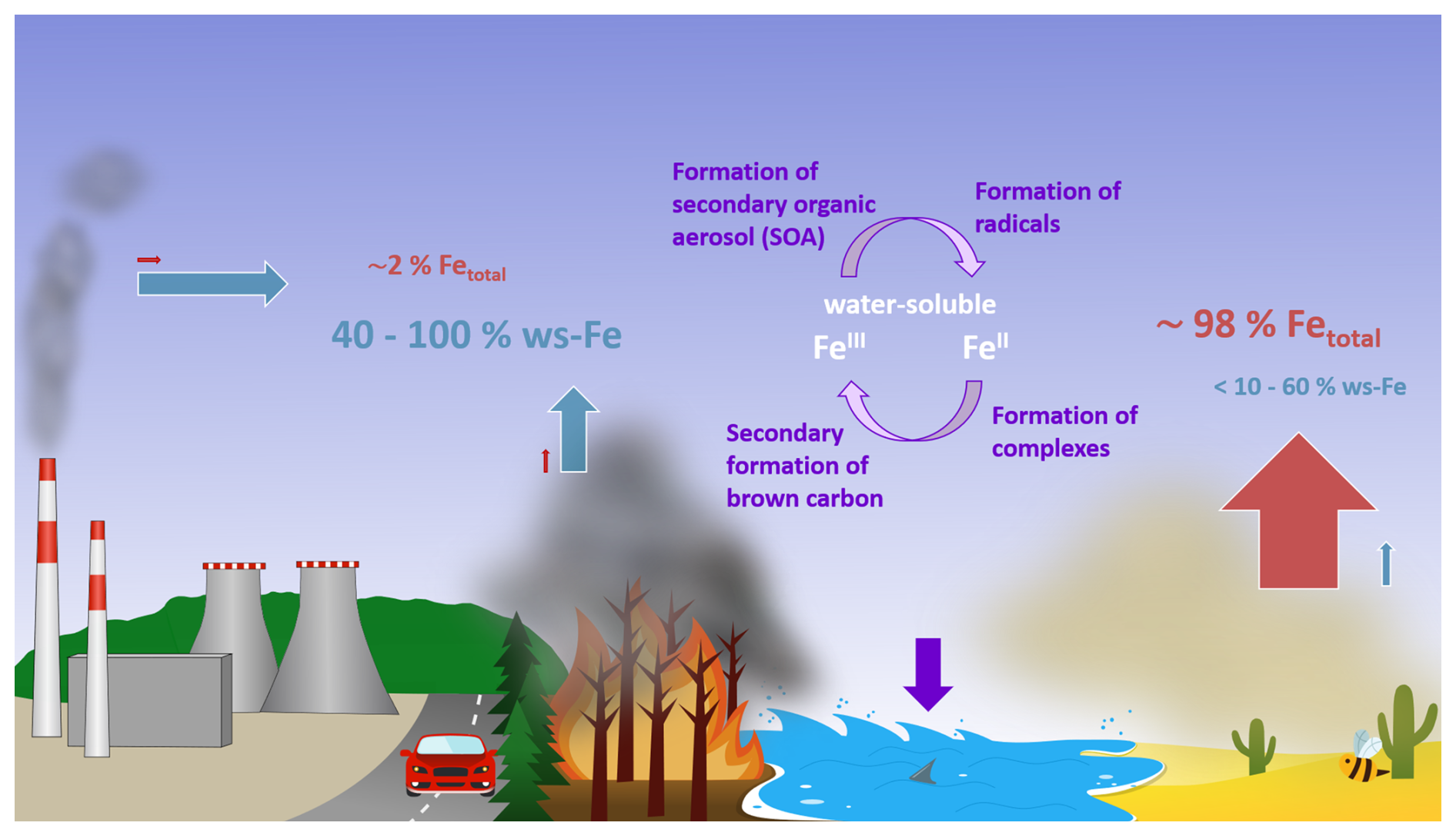
Furthermore, airborne soluble iron is present in either Fe(II) or Fe(III) and can thus participate in multiple atmospheric processes altering the chemical composition of aerosols (Al-Abadleh, 2024; Pehkonen et al., 1993). For example, previous studies have shown that soluble iron impacts the formation of secondary organic aerosol (Lüchtrath et al., 2024; Chu et al., 2017), and, depending on the oxidation state, light conditions and the presence of hydrogen peroxide (H₂O₂) can lead to the formation of light-absorbing particles by reacting with phenolic precursors (Lüchtrath et al., 2025; De Haan et al., 2024; Hopstock et al., 2023; Slikboer et al., 2015), thus having a direct impact on the Earth's radiative budget.

In the aqueous phase, iron acts as a major catalyst for hydroxyl (OH) radical formation through Fenton (Fe(II) + H₂O₂) and photo-Fenton (Fe(III) + light + H₂O₂) reactions, thus enhancing the oxidation capacity of aerosol particles in atmospheric droplets (Tilgner and Herrmann, 2018; Herrmann et al., 2015; Arakaki and Faust, 1998; Zepp et al., 1992; Fenton, 1894).

On a global scale, mineral dust is the primary source of atmospheric iron; Ito and Shi (2016) estimated that it contributes about 98 % of the total atmospheric iron budget. Freshly emitted dust exhibits very low iron solubility (Longo et al., 2016; Mahowald et al., 2009; Luo et al., 2005). During atmospheric transport, Fe-bearing minerals can dissolve through three main pathways, which are proton-promoted, ligand-promoted, and reductive dissolution (Al-Abadleh et al., 2024; Chen and Grassian, 2013; Rubasinghege et al., 2010). These three mechanisms are influenced by various factors like pH, particle size, presence of solar radiation, crystallinity of the Fe-bearing mineral. and the Fe organic complexes (Liu et al., 2022; Meskhidze et al., 2017; Paris and Desboeufs, 2013; Journet et al., 2008). Over the last few decades, research has consistently demonstrated that iron dissolution rates are highest under acidic conditions (pH < 4), particularly when exposed to solar radiation and oxalate (e.g. Chen and Grassian, 2013) with nanometre-sized, amorphous iron, especially from combustion sources (e.g. Baldo et al., 2022; Ito et al., 2019).

Under typical environmental conditions, Fe(II) starts to hydrolyse at pH > 8, whereas Fe(III) hydrolysis begins already at pH > 3 (Langmuir, 1997). Atmospheric aerosols and cloud and fog droplets exhibit acidity spanning approximately 5 pH units (Pye et al., 2020). Typical pH values for cloud droplets range from 3 to 6 (Pye et al., 2020). However, most cloud droplets do not precipitate as rain; instead, they evaporate, leaving a thin residual water film around dust particles. The wet aerosols can have aqueous-phase pH values below 2 (Pye et al., 2020). Shi et al. (2015) simulated the cycling of Fe-containing particles between wet aerosols (pH 1–2) and cloud droplets (pH 5–6). They found that acidic wet aerosol conditions promote rapid dissolution of low soluble Fe-containing particles, whereas, at higher pH levels, in cloud droplets, precipitation of Fe-rich nanoparticles is favoured, which can rapidly re-dissolve upon droplet evaporation. The authors further emphasized that the duration of the acidic aerosol stage increases the amount of soluble iron.

As illustrated in Fig. 1, combustion processes like biomass burning, industrial production, and also traffic contribute only a few percent to the total amount of atmospheric iron (Ito and Shi, 2016; Luo et al., 2008) but possibly make up 40 %–100 % of the total soluble Fe fraction (Ito, 2015; Sholkovitz et al., 2009; Luo et al., 2008). The concentrations of dissolved iron in fog and cloud water can therefore vary locally depending on environmental conditions and the iron emission source, ranging between 0.002 and 647 µmol L⁻¹ (Bianco et al., 2020; Deguillaume et al., 2005).

Figure 1 Sources, sinks, and processes of atmospheric water-soluble iron.

In atmospheric-science literature, solubility is often defined as the percentage of dissolved Fe, measured in the filtrate after passing through a 0.2–0.45 µm pore size filter relative to the total Fe content in the bulk aerosol sample (Shi et al., 2012). Because the concentration of Fe in the filtrate (and, thus, its measured solubility) depends on pH, we use the term “water-soluble (ws) Fe” in this study. This includes Fe measured both in neutral water (Seradest, pH 6.5) and under slightly acidic conditions (pH 4.5), which simulate cloud water environments.

A common method to determine water-soluble Fe(II) (ws-Fe(II)) in ambient aerosols (Kuang et al., 2020; Oakes et al., 2010; Rastogi et al., 2009) spectrophotometrically is the reaction between dissolved Fe(II) and ferrozine, leading to the formation of a stable magenta-coloured complex developed by Stookey (1970). The reduction of dissolved Fe(III) to Fe(II) by a reductant like hydroxyl ammonium hydrochloride (HA) enables the determination of total ws-Fe and has been extensively used (Lei et al., 2023; Majestic et al., 2006; Stookey, 1970). The applied reduction time varies from some minutes (Lei et al., 2023; Kuang et al., 2020) to several hours (Yang et al., 2021).

The principle of flow injection analysis (FIA) first introduced by Nagy et al. (1970) is the precise introduction of sample volumes into a continuous, bubble-free stream, enabling automated analyses that are fast, accurate, and widely applicable. FIA setups have been used to determine ws-Fe(II) and total ws-Fe of different origins, such as natural water, waste water, potato leaves, or human hair (e.g. Pullin and Cabaniss, 2001; Pascual-Reguera et al., 1997).

Aerosols are typically collected on filter for 12–24 h and analysed offline afterwards. The offline analysis limits the investigation of time-resolved variability in the concentrations and speciation of ws-Fe. Furthermore, the redox state of iron can change during collection and filter storage. Rastogi et al. (2009) developed the first online technique for determining water-soluble Fe(II) in ambient aerosols using a particle-into-liquid sampler coupled with a continuous-flow ferrozine method.

Building on the work of Rastogi et al. (2009), we present an online method combining FIA and particle-into-liquid sampling to quantify ws-Fe(II), total ws-Fe, and thereby ws-Fe(III), advancing insights into ws-Fe sources, processes of Fe dissolution, and the role of iron chemistry in atmospheric processes (Fig. 1).

2 Methods

2.1 Chemicals and solution preparation

Except for the glass volumetric flasks, only plastic bottles and beakers were used to avoid iron cross-contamination. All vessels were cleaned by soaking in 0.03 M HNO₃ and rinsed with Seradest water (Seradest S750, Veolia Water Technologies, Germany). The 0.03 M HNO₃ was prepared from bidistilled water and HNO₃ (65 %, Suprapur, Merck, Germany). A 0.8 mM HNO₃ solution was prepared to achieve a pH of 3–3.5, while a 0.04 mM HNO₃ solution was used to obtain a pH of 4.5. All working standards and solvents for the FIA system were freshly prepared daily. The iron working standards (0.5–50 µg L⁻¹) were prepared by dilution of a 1 g L⁻¹ dissolved Fe(II) stock solution (acidified to pH1 by HCl) of FeSO₄ ⋅ 7H₂O (≥ 99 % p.a., Carl Roth GmbH, Germany) and a 1 g L⁻¹ dissolved Fe(III) stock solution (acidified to pH1 by HCl) of NH₄Fe(SO₄)₂ ⋅ 12H₂O (≥ 98 %, Carl Roth GmbH, Germany). Ferrozine solutions were prepared by dissolving 133 mg 3-(2-pyridyl)-5,6-diphenyl-1,2,4-triazine-4^′,4^′′-disulfonic acid sodium salt (ferrozine, iron reagent, hydrate, 95+ %, pure, Thermo Scientific Chemicals, Germany) in 100 mL Seradest water, resulting in a 2.7 mM solution. As a reduction reagent, 19.3 mg hydroxylamine hydrochloride (99.9 %, Thermo Scientific Chemicals, Germany) was dissolved in 50 mL Seradest water. For cleaning the FIA system and the liquid waveguide capillary cell (LWCC), methanol, 2 M HCl, and 2 % Hellmanex (Hellma Analytics GmbH & Co. KG, Germany) were used.

2.2 Definition of water-soluble iron

The lack of a standardized protocol for determining trace metal solubility, including Fe, has been widely discussed in the literature (e.g. Tang et al., 2025; Perron et al., 2020; Meskhidze et al., 2016). Several studies have demonstrated that leaching or extraction procedures, including different chemical compositions and pH values of the solutions, as well as different contact times, strongly influence the measured metal's solubility (e.g. Li et al., 2023; Tang et al., 2025; Perron et al., 2020; Meskhidze et al., 2016). Most comparative studies investigating the effect of leaching solutions on iron solubility have used ultrapure water or organic buffers such as formate or acetate with a pH of around 4.3 (e.g. Li et al., 2023; Perron et al., 2020; Majestic et al., 2006).

As no standard protocol exists, a variety of operational terms have been used in the literature to describe experimentally mobilized aerosol trace element fractions, including “soluble”, “labile”, “leachable”, “dissolved”, “readily accessible”, “bioaccessible”, and “bioavailable”, as summarized by Tang et al. (2025). The use of different extraction or leaching approaches and definitions complicates direct comparison of reported iron solubility and soluble-iron concentrations across studies.

This study focuses on the determination of the iron fraction which is soluble in Seradest water (pH 6.5), used as a near-neutral reference condition, and Seradest water adjusted to pH 4.5 with HNO₃, providing mildly acidic, low-ionic-strength aqueous conditions representative of cloud water acidity while minimizing additional chemistry introduced by adding buffering agents. The pH of the aqueous phase can vary widely, ranging from highly acidic conditions (pH < 0) in deliquesced aerosols to neutral pH in rain and fog water (e.g. Pye et al., 2020; Herrmann et al., 2015). As discussed above, the solubility of atmospheric iron depends on particle size, chemical composition, photochemical activity, and atmospheric processing, as well as on pH. To allow a clearer interpretation of our data, we therefore use the term “water-soluble iron” throughout this study, emphasizing that the reported values represent the fraction of iron that is soluble under neutral and mildly acidic aqueous conditions relevant to cloud water, fog water, and rainwater.

A key advantage of the online approach is the high temporal resolution of the measurements; however, the method is based on short extraction and reaction times for both ferrozine and the reducing reagent hydroxylamine (HA), as will be discussed in Sect. 3.1.1. Consequently, the quantity reported as ws-Fe(II) is operationally defined by the reaction time of dissolved Fe(II) with ferrozine. The term “total ws-Fe” refers to the amount of Fe detected as dissolved Fe(II) after the addition of HA, which reduces dissolved Fe(III) to Fe(II) prior to complexation with ferrozine.

2.3 Online analysis system

A measurement setup consisting of a commercially available particle-into-liquid sampling unit and a custom-built flow injection analysis (FIA) system with a liquid waveguide capillary cell (LWCC) was developed to detect, in online mode, the concentration and oxidation state of water-soluble atmospheric soluble iron. Two commercially available sampling units were used: the Metrohm AeRosol Sampler (MARS; Metrohm Process Analytics, Filderstadt, Germany) and the Particle-Into-Liquid Sampler (PILS BMI 4002, Brechtel Manufacturing Inc., USA). Concentrations of ws-Fe(II) and total ws-Fe were quantified spectrophotometrically by the ferrozine method. Ferrozine and dissolved Fe(II) form a complex with a characteristic absorbance maximum at λ = 562 nm (Stookey, 1970). Total ws-Fe was determined after reduction of dissolved Fe(III) to Fe(II) using hydroxylamine hydrochloride (HA) as a reduction reagent. A scheme of the setup is shown in Fig. 2. All dimensions and flow parameters are listed in Table 1. The system components will be explained in more detail in the following sections.

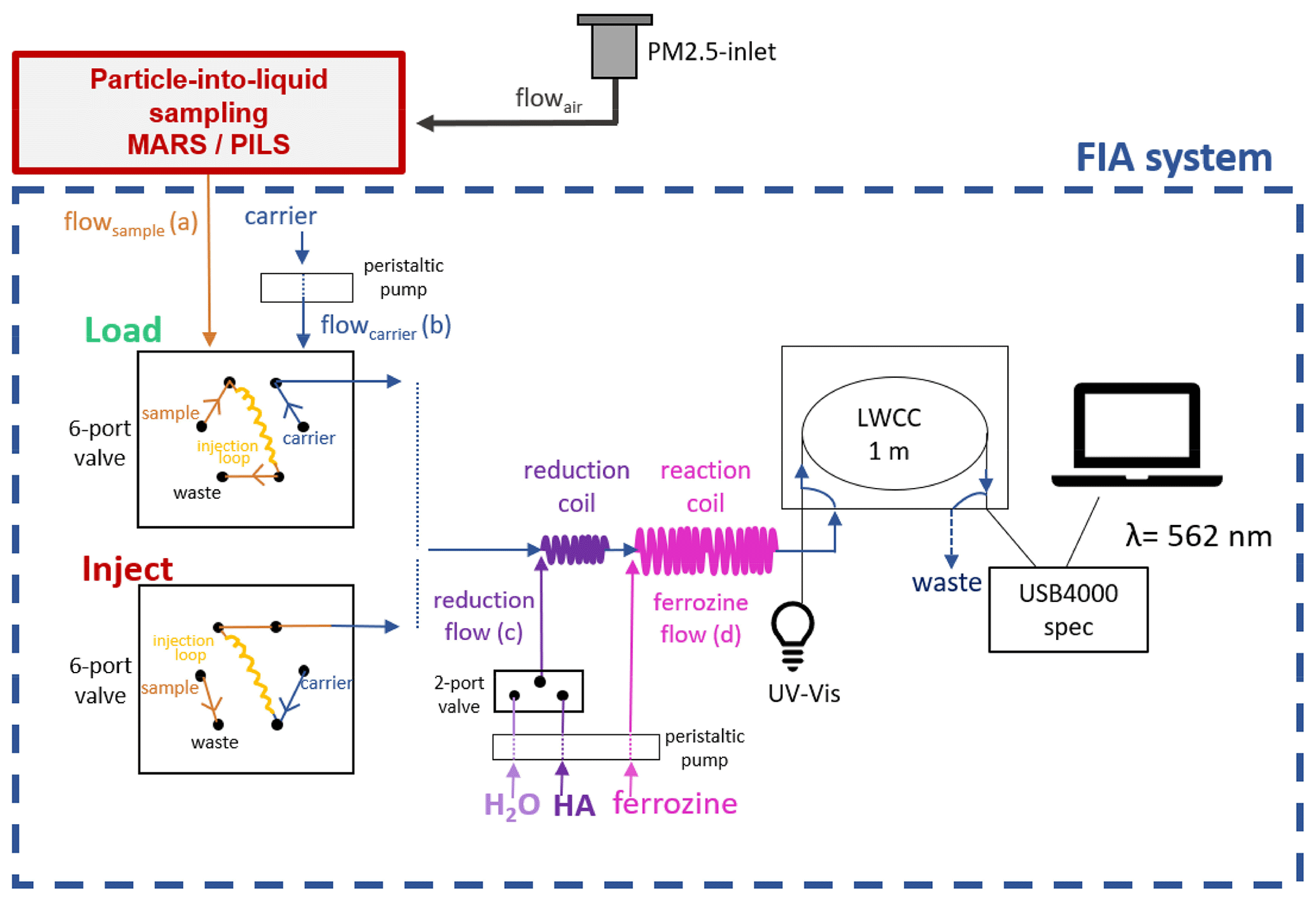
Figure 2 Schematic diagram of the measurement setup in detail. During LOAD mode, the aerosol sample solution is transferred into the injection loop of the six-port valve, while the carrier stream flows through the FIA system. After the injection loop is filled (10 min for the MARS-FIA and 12 min for the PILS-FIA), the automated six-port valve switches to INJECT mode. In INJECT mode, the carrier stream is directed through the injection loop, thereby pushing the sample towards the reaction coil of the FIA system. The sample is first transferred into a T piece connected to a two-port valve, where HA or H₂O are added alternately to the sample stream before entering the reduction coil. After passing the reduction coil, the sample stream enters a second T piece where ferrozine is added prior to the reaction coil. Following the reaction coil, the sample enters the LWCC coupled to a spectrophotometer, where absorbance is measured.

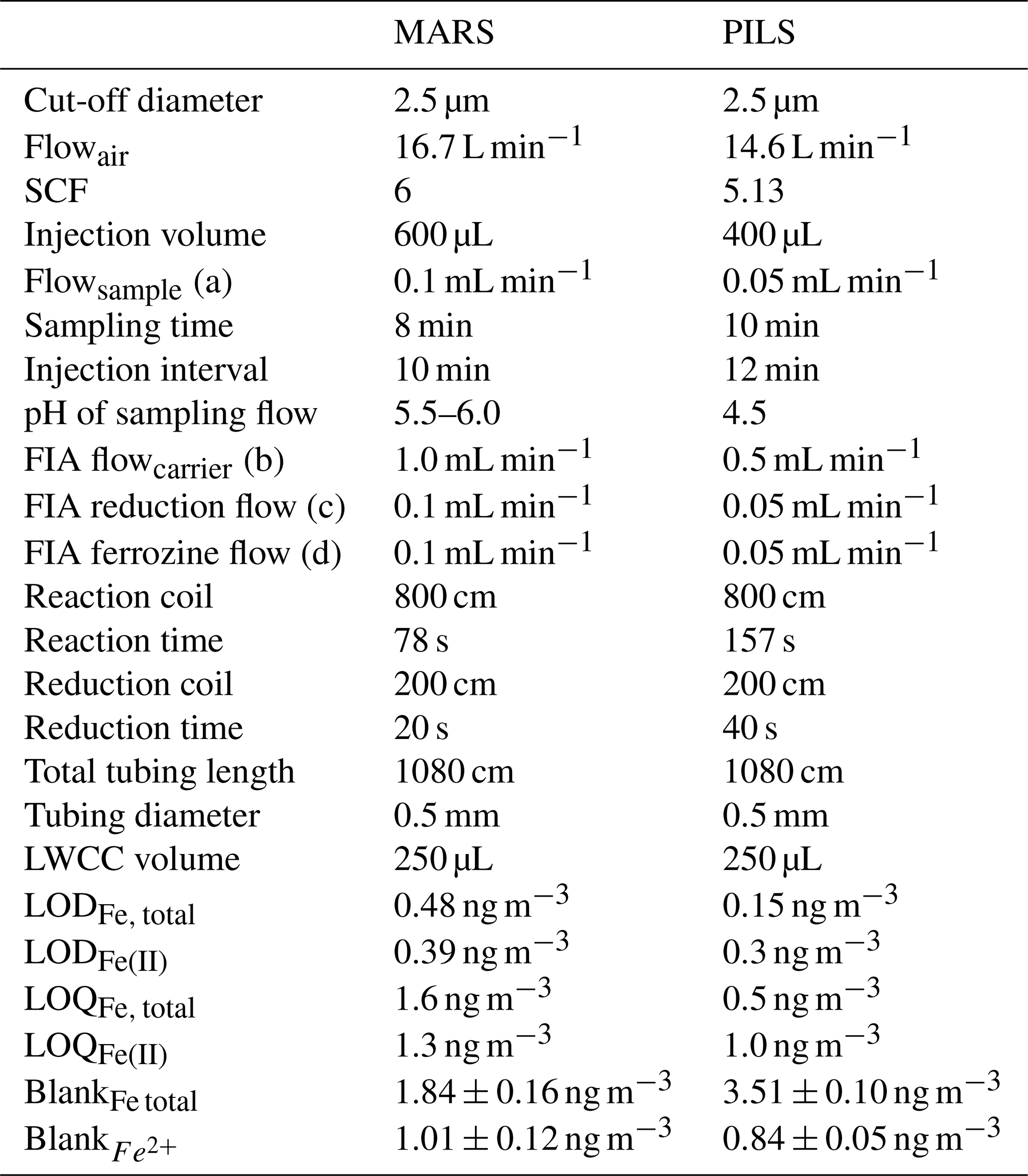
Table 1 Overview of dimensions and operational parameters for MARS- and PILS-FIA systems.

2.3.1 Particle-into-liquid sampling units

Particle-into liquid sampling units are designed to enable an online analysis of ambient aerosol bulk composition. The basic principle is based on particle growth into droplets through the supersaturation of water vapour, which are then collected in a liquid solution (e.g. Stieger et al., 2018; Weber et al., 2001). The Metrohm AeRosol Sampler (MARS) is part of the commercial Monitor for AeRosols and Gases in ambient Air (MARGA, Metrohm, Applikon, Netherlands). Both MARGA and PILS measurements were conducted in several studies (e.g. Zeng et al., 2021; Stieger et al., 2019) and are thus validated approaches for the online determination of water-soluble aerosol compounds.

Metrohm AeRosol Sampler (MARS)

The MARS sampler was connected to a PM_2.5 inlet. The airflow of 1 m³ h⁻¹ is regulated by the usage of a critical orifice. The air flow passes the Wet Rotator Denuder (WRD), which removes soluble gases from the air stream. Aerosols will not be absorbed but follow the air stream due to their inertia. After having passed the WRD, the air stream enters the Steam Jet Aerosol Collector (SJAC) where supersaturated water steam is introduced by a steamer. In the steamer chamber, the particles grow by deliquescence. Due to their inertia, the grown particles are separated by the cyclone and collected in the 1.2 mL sampling volume on the bottom of the SJAC. The liquid sampled is continuously transferred through a 0.45 µm syringe filter into the injection loop of the FIA system. The sample flow to the FIA system was adjusted to 0.1 mL min⁻¹. The sample concentration factor (SCF) describes the ratio between the concentration in the atmosphere (c_air) and the liquid sample (c_sample) (Eq. 1). The MARS-FIA system had an SCF of 6. As no internal standard was used, no dilution factor was applied.

$$\begin{array}{}\text{(1)}& c_{\mathrm{air}}\left[\mathrm{ng}{\mathrm{m}}^{-\mathrm{3}}\right]=c_{\mathrm{sample}}\left[\mathrm{\mu }\mathrm{g}{\mathrm{L}}^{-\mathrm{1}}\right]\cdot \text{SCF}\end{array}$$

Particle-Into-Liquid Sampler (PILS)

The PILS BMI4002 is a modification of the PILS instrument described by Weber et al. (2001). Its setup and operation mode were described in detail by Sorooshian et al. (2006). The PILS was used in online mode and operated at an air flow rate of 14.6 L min⁻¹ with a 2.5 µm diameter-cut cyclone at the inlet. No denuders were installed. In the condensation chamber, the ambient air mixes with steam, leading to supersaturation and, therefore, particle activation. The activated particles grow to > 1 µm diameter before they reach the impaction plate (Sorooshian et al., 2006). A wash flow of 0.065 mL min⁻¹ transports the impacted droplets down the impactor plate, from which they are transferred to the FIA system at a sample flow rate (Flow_Sample(a)) of 0.05 mL min⁻¹. The pH of an average droplet can be expected to be 5.6 (Ma, 2004; Sorooshian et al., 2006). To test whether Fe solubility is increased by lowering the pH of the sample, the wash flow was acidified slightly to pH 4.5 using 0.04 mM HNO₃. During particle collection, liquid from the droplets and the transport flow solution can dilute the sample. Additionally, water condenses on the impaction plate. Orsini et al. (2003) quantified this additional water as 5 to 20 µL  min⁻¹. As no internal standard was used in this study and the wash flow was 1.3 times higher than the sample flow, a dilution factor of 1.5 was applied, assuming an average additional condensed-water contribution of 10 µL min⁻¹. The SCF for the PILS system was 5.13.

Blank measurements of both sampling units were conducted regularly by directing the air flow through a HEPA zero filter (HEPA-CAP, Whatman, UK). The filter was connected for 1 h prior to measurement. Blank values were then determined from the subsequent 2 h of sampling. The limit of quantification (LOQ) was defined to be 10 times the standard deviation of the blank values, and the limit of detection (LOD) was defined to be 3 times this value (Eqs. 2 and 3), and both were determined for ws-Fe(II) and total ws-Fe.

$$\begin{array}{}\text{(2)}& {\displaystyle }\text{LOD}=\mathrm{3}\cdot {\mathit{\sigma }}_{\mathrm{blanks}}\text{(3)}& {\displaystyle }\text{LOQ}=\mathrm{10}\cdot {\mathit{\sigma }}_{\mathrm{blanks}}\end{array}$$

2.3.2 Flow injection analysis unit

A three-line flow injection analysis system was developed to quantify soluble iron in liquid samples using spectrophotometric detection. Ferrous iron (Fe(II)) forms a stable magenta complex with ferrozine, which absorbs at 562 nm, enabling its detection. This method was originally introduced by Stookey (1970). A previous reduction of the present dissolved Fe(III) further enables the determination of the total soluble-iron fraction.

$$\begin{array}{}\text{(4)}& \text{total ws-Fe}=\text{ws-Fe(II)}+\text{ws-Fe(III)}\end{array}$$

This FIA system includes two peristaltic pumps (ISMATEC, IPS 8), a common six-port valve used in HPLC systems (BESTA, Germany) with an injection loop, a two-way switching pinch valve (ASCO S306.02-Z530A), a 2 m reduction coil with an inner diameter of 0.5 mm and a volume of 0.4 mL, an 8 m reaction coil with an inner diameter of 0.5 mm and a volume of 1.6 mL, a UV–Vis light source (DH-2000-BAL, Ocean Optics, Germany), a USB Spectrophotometer (USB4000-XR1-ES, Ocean Optics, Germany), and a liquid waveguide capillary cell (LWCC 3100, World Precision Instruments, Friedberg, Germany, 100 cm pathlength, 250 µL internal volume, 0.5 mm inner diameter) (see Fig. 2). The valve circuits of the six-port valve and the two-way pinch valve were controlled with a microcontroller (Arduino Nano). Software for data acquisition was written in LabView 2017 based on Ocean Optics USB4000 code.

During LOAD mode of the six-port valve, a continuous sample flow from the MARS or PILS system was directed into the injection loop (600 µL for MARS and 400 µL for PILS), both exceeding at least 1.5 times the volume of the LWCC (see Fig. 2). Due to the different sample flow rates (MARS: 0.1 mL min⁻¹; PILS: 0.05 mL min⁻¹), a smaller injection loop volume was used for the PILS–FIA system compared to the MARS–FIA system to achieve a comparable injection time resolution. While the sample solution filled the injection loop, the carrier stream passed through the FIA system, providing the baseline signal. The carrier flow rate was set to 1.0 mL min⁻¹ for the MARS–FIA system and 0.5 mL min⁻¹ for the PILS–FIA system. The pH of the carrier stream was adjusted to match the pH of the respective sample flow (pH 6.5 for MARS and pH 4.5 for PILS).

To ensure complete filling of the injection loop, sampling times of 8 min for the MARS–FIA system and 10 min for the PILS–FIA system were applied. Accordingly, the six-port valve switched from LOAD to INJECT mode after 8 min (MARS–FIA) and 10 min (PILS–FIA). During INJECT mode, the sample solution was injected into the carrier stream (see Fig. 2). At the first mixing point, either hydroxylamine hydrochloride (HA) solution or Seradest water (H₂O) was introduced into the carrier stream via a two-port switching valve (flow rate ratio carrier: HA $/$ H₂O = 10 : 1). The injection valve was switched back to LOAD mode after 2 min so that fresh extractant solution was filled into the loop, thereby decreasing the waiting time for the subsequent injection and increasing the sampling frequency.

For each LOAD–INJECT cycle, only one reagent was added into the sample stream. The addition of HA and H₂O was alternated between consecutive LOAD cycles, such that HA was added during one cycle and H₂O was added during the subsequent cycle. The two-port valve was switched during each LOAD mode after the peak of the previous sample had been fully detected. Because the addition of HA caused a baseline shift, the switching between HA and H₂O was carefully timed to occur between two consecutive peaks.

After passing the first mixing, the sample stream entered the reduction coil, where dissolved Fe(III) was reduced to Fe(II) only in the presence of HA. At the second mixing point, ferrozine was introduced into the sample stream (flow rate ratio (ferrozine : carrier) of 1 : 10) before it entered the reaction coil. In previous online systems for ws-Fe(II) detection, ferrozine concentrations around 5 mM were commonly used (e.g. Rastogi et al., 2009; Majestic et al., 2006), typically added to the sample at a 1 : 10 ratio. In this study, a lower ferrozine concentration of 2.7 mM was sufficient for complete complexion of dissolved Fe(II) while also reducing chemical consumption. Experiments with dissolved Fe(II) standard solutions indicated that 95 % of the maximum absorbance of the magenta-coloured Fe(II)–ferrozine complex was already reached after 70 s, allowing short reaction times (∼ 80 s for MARS-FIA and ∼ 160s for PILS-FIA). Due to the short reaction time, the reduction of dissolved Fe(III) by ferrozine alone was not observed, as has been reported in previous studies (Murray and Gill, 1978). As the pH of the sample flow is not expected to be below pH 4.5, which is in the working range of ferrozine as a complexing agent (Zhang et al., 2001; Stookey, 1970), no buffer was used. After passing the reaction coil, the sample enters the LWCC. To prevent the formation of air bubbles due to outgassing, a PTFE capillary (0.5 mm inner diameter, 350 mm length; Metrohm AG, Germany) was attached to the outlet of the LWCC as it increases the back pressure within the LWCC. The sample absorbance was determined at λ = 562 nm relative to λ = 700 nm. The average baseline was determined over a 75 s interval, from 2 min to 45 s before the peak, and subtracted from the signal. Quantification using peak height gave better precision than using peak area and was therefore applied in this study. All values were subsequently corrected for blank measurements.

2.3.3 Calibration and daily maintenance

The FIA system was regularly calibrated with 3–5 dissolved Fe(II) standards ranging from 0.5 to 40 µg L⁻¹, freshly diluted from a 1 g L⁻¹ acidified stock solution. Daily calibration was performed with a 5 µg L⁻¹ Fe(II) standard. While Fe(II) is typically stabilized in 0.01 M HCl (Zhang et al., 2001) due to a slower oxidation rate in acidic conditions (Millero et al., 1987), neutral pH standards were used here to match sample conditions and yielded reproducible results. For each measurement sequence, a single dissolved Fe(III) standard of pH 3.5 was regularly used to assess reduction efficiency. The standards showed improved stability and reproducibility when acidified to pH 3.5 compared to neutral pH conditions as dissolved Fe(III) hydrolysis occurs at pH > 3, while dissolved Fe(II) hydrolysis occurs at pH > 8 (Langmuir, 1997). An optimum pH range of 4–9 for the Fe(II)–ferrozine complex formation was stated by Stookey (1970), but calibrating with dissolved Fe(II) standards of pH 3.5 gave the same results compared to calibrating with a neutral pH solution, underlining that the ferrozine method also works at pH 3.5. To prevent the accumulation of the Fe–ferrozine complex on the LWCC inner wall, the LWCC was cleaned daily with 2 % Hellmanex, methanol, and 2 M HCl. FIA tubing was washed with 2 M HCl regularly to prevent the precipitation of iron oxides within the tubing.

2.4 Test experiments and instrument evaluation

2.4.1 Test experiments

Following the development of the FIA system, the setup was connected to MARS and tested during a 2-week measurement campaign in June 2024 in Berlin, Germany. The system was deployed inside a measurement container located at the main campus of Technische Universität (TU) Berlin, close to the six-lane road “Straße des 17. Juni”. During the campaign, particle size distributions were measured using an ELPI+ (Dekati, Finland), and equivalent black carbon (BC) concentrations were determined with an aethalometer (MA200, AethLabs, USA). After this initial test campaign, the setup was optimized by adjusting the pH of the extraction medium. A second 1-week campaign was conducted in March 2025 on the terrace of an institute building at the TU Berlin campus. This time, a PILS was used as the sampling unit, with an acidified sample flow at pH 4.5. BC concentrations were measured again using the aethalometer MA200. PM_2.5 concentrations were obtained from the background monitoring stations in districts of Berlin (i.e. Wedding, Neukölln, and Mitte), which are part of the Berlin Air Quality Monitoring Network (BLUME).

2.4.2 Offline measurement

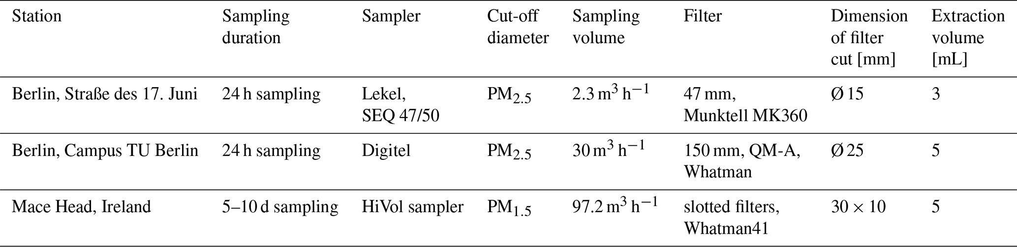
To evaluate the results from the online instruments, filter samples were collected during the test field campaigns in Berlin. Additional filter samples were taken at a contrasting location to assess potential application environments: Mace Head, Ireland (autumn 2024), representing background North Atlantic marine air (O'Connor et al., 2008). As different filter samplers, air volumes, filter types, and diameters were used at the different locations, all parameters are listed in Table 2. The filters from Mace Head were stored frozen and transported to Berlin in a frozen state. The filters in Berlin were stored at room temperature and in the dark before extraction.

Iron solubility is strongly influenced by pH – lower pH values lead to increased solubility (Liu and Millero, 2002, 1999). Based on the mean pH values reported by Pye et al. (2020) for 93 studies at 48 European locations between 1988 and 2018, the average pH of cloud water in Europe is approximately 4.5. This value lies within the optimal pH range of the ferrozine method and was therefore selected for comparison with neutral pH (pH 6.5) conditions.

To assess the effect of pH on ws-Fe(II) concentration, filter cuts were extracted in Seradest water at pH 4.5 and at pH 6.5 for 1 h in a horizontal shaker. Different cut sizes were used depending on the used particle collector (see Table 2). The extracts were filtered through a 0.45 µm polyamide syringe filter (Chromatographie Handel Mueller, Germany) before they were injected into the FIA system for ws-Fe(II) and total ws-Fe determination. Samples were directly analysed after extraction to minimize hydrolysis and precipitation of dissolved Fe(III), as well as oxidation of Fe(II) to Fe(III).

Table 2 Summary of filter sampling parameters at the different locations.

Extraction time and extraction pH vary across different studies published; for example, Chen and Siefert (2003) report that a maximum concentration of labile Fe was reached after 90 min at pH 4.5. To evaluate extraction efficiency at pH 4.5 for the much shorter extraction times typical of particle-into-liquid sampling units (only a few minutes), filters from the second campaign were extracted for 1, 5, 10, and 30 min. The total ws-Fe(II) concentration was determined directly after extraction using the FIA system, and extraction efficiency was then calculated.

3 Results and discussion

3.1 Characteristics of the FIA system

3.1.1 Calibration and limit of quantification

Based on measurements of calibration standards and system blanks, the linear working range, the sensitivity, the limit of detection (LOD), and the limit of quantification (LOQ) of the FIA system were obtained.

A universal calibration curve from 0.5 to 40 µg L⁻¹ dissolved Fe(II) was determined as an average linear regression of 10 individual calibration measurements taken over the course of 1 year (Table A1 in the Appendix), based on measurements performed on different days in the laboratory and under varying conditions in the field, including minor fluctuations in flow rates and changes in pump tubing. The individual linear regression slope values ranged from 0.0206 to 0.0280 (1/µg L⁻¹), with an average of 0.0242 ± 0.0024 (1/µg L⁻¹). The intercept was −0.0023 ± 0.0076, and R² was 0.996. The low standard deviation of the slopes (< 10 %) demonstrates good reproducibility for calibration slopes, highlighting the robustness of the system under varying operational conditions and confirming its suitability for field deployment. Reduction efficiency was tested with single dissolved Fe(III) standards of pH 3.5 and showed high efficiency, varying between 80 % and 117 % relative to dissolved Fe(II) when standards were freshly prepared. A decrease in reduction efficiency was observed with increasing age of the dissolved Fe(III) standards, likely due to the formation of hydrolysed Fe(III) species which are not rapidly reduced by HA. This observation highlights that, under the short reduction times in the FIA system, less reactive or less reducible Fe(III) species may not be fully reduced. Previous studies have used HA as reducing solution in flow injection systems applying very short reaction times (HA and ferrozine together) of approximately 1 min (e.g. Pullin and Cabaniss, 2001; Teixeira and Rocha, 2007). In the presented systems, the reduction times were 20 s for the MARS and 40 s for the PILS system. The reaction times with ferrozine were 78 s for the MARS and 157 s for the PILS system (Table 1). Therefore, the total time for the reduction of dissolved Fe(III) into Fe(II) was 98 s for the MARS and 197 s for the PILS system. Pullin and Cabaniss (2001), using an acetate buffer carrier of pH 4.0 and a reaction temperature of 65 °C, reported 100 % reduction efficiency by adding acetic acid into the carrier and colour reagent, suggesting that the acetate buffer forms a complex with the dissolved Fe(III). As no buffer solution was used in the present FIA apparatus, the addition of acetic acid had no effect on reduction efficiency when injecting aged Fe(III) standards. Heating of the reduction coil in a water bath as reported by Pullin and Cabaniss (2001) was not applied to reduce the technical complexity for a system which is intended to run continuously for a long period of time. Similarly, heating was not applied in many other FIA systems designed for ws-Fe(II)/(III) determination (e.g. Attiyat et al., 2011; Teixeira and Rocha, 2007).

Luther et al. (1996) reported incomplete reduction of dissolved Fe(III) by HA in the presence of humic-like substances.

To acknowledge this limitation imposed by the operationally given reduction time, further on we use the term reducible Fe(III) instead of ws-Fe(III). This also underlines that total-ws Fe is defined by the kinetics of the FIA system and might also underestimate the total ws-Fe concentration compared to studies with longer reduction times.

The average blank concentrations from the test field campaigns (n = 2) are listed in Table 1. Generally, the mean blank concentrations of total ws-Fe (MARS-FIA: 1.84 ng m⁻³; PILS-FIA: 3.51 ng m⁻³) are higher compared to the mean blank concentrations of ws-Fe(II) (MARS-FIA: 1.01 ng m⁻³; PILS-FIA: 0.84 ng m⁻³). The PILS-FIA-system shows higher blank values for total soluble iron than the MARS-FIA system. An advantage of the MARS is the fast and simple washing procedure as the SJAC can quickly be dismantled and cleaned in isopropanol in an ultrasonic bath.

The lowest LOD with 0.15 ng m⁻³ was determined for total ws-Fe using the PILS-FIA setup (Table 1). The highest LOD with 0.48 ng m⁻³ (Table 1) was determined for total ws-Fe using the MARS-FIA setup. The LOQ from the blank measurement of total ws-Fe was 1.6 ng m⁻³ for the MARS-FIA and 1.0 ng m⁻³ for the PILS-FIA (Table 1). The blank uncorrected LOQ for the MARS-FIA system was 2.7 ng m⁻³, which corresponds to 0.45 µg L⁻¹, and 5.1 ng m⁻³ for the PILS-FIA system, which corresponds to 1.15 µg L⁻¹. These liquid concentrations are at the lower end of the calibration range.

3.1.2 Effect of pH and extraction time

As iron solubility is directly influenced by pH, which typically ranges between 3 and 6 in cloud water (Pye et al., 2020), filters were extracted at a near-neutral reference pH (6.5) and cloud-water-related pH (4.5) (see Sect. 2.4.2).

At pH 6.5, the lowest ws-Fe concentrations were found at Mace Head, Ireland (Table 3, filters C1–C5), with ws-Fe(II) ranging from < LOQ to 0.04 ng m⁻³. Total ws-Fe concentrations were only slightly higher (LOQ–0.06 ng m⁻³), resulting in ws-Fe(II) $/$ total ws-Fe ratios of around 0.8. These high ratios indicate that nearly all water-soluble Fe was present as dissolved Fe(II).

When extracted at pH 4.5, both ws-Fe(II) and total ws-Fe concentrations increased, reaching 0.07–0.16 and 0.13–0.29 ng m⁻³, respectively. The relative increase was higher for total ws-Fe than for ws-Fe(II), leading to a lower ws-Fe(II) $/$ total ws-Fe ratio of 0.45–0.70. This indicates that, under slightly acidic conditions, more reducible Fe(III) compounds dissolved than Fe(II), as expected from the enhanced solubility of Fe(III) oxides and Fe(III) hydroxides at lower pH (e.g. Balsamo Crespo et al., 2023; Langmuir, 1997; Pye et al., 2020). The very low ws-Fe(II) and total ws-Fe concentrations are evidence of the clean air and pristine marine conditions at Mace Head.

In contrast to the clean marine air masses sampled at Mace Head, Berlin urban air is strongly influenced by anthropogenic activity, which is reflected in higher concentrations of both ws-Fe(II) and total ws-Fe (Table 3). During the second test campaign in winter 2025 (Filters B5–B9), extraction at pH 6.5 yielded ws-Fe(II) concentrations between 1.1 and 7.5 ng m⁻³ and total ws-Fe between 3.2 and 16.47 ng m⁻³. The resulting ws-Fe(II) $/$ total ws-Fe ratios of 0.22–0.46 indicate that a large fraction of water-soluble iron was present as reducible Fe(III) rather than ws-Fe(II). When filters were extracted for 1 h at pH 4.5, concentrations increased substantially: ws-Fe(II) increased to 10.78–21.63 ng m⁻³, and total ws-Fe increased to 11.76–5.47 ng m⁻³, resulting in higher ws-Fe(II) $/$ total ws-Fe ratios of 0.68–0.92. This result indicates that, under mildly acidic, cloud-water relevant conditions, a large fraction of the dissolved iron is present as Fe(II). This enrichment may reflect the mobilization of Fe that has previously undergone ligand-mediated dissolution and redox processing in the atmosphere, where organic ligands such as oxalate are known to increase iron dissolution by complexation and to facilitate photoreduction of Fe(III) to Fe(II) under mildly acidic conditions (Shi et al., 2012). In addition, complexation with organic ligands has been shown to stabilize dissolved Fe(II) in rainwater of pH 4.5 (Kieber et al., 2005). Overall, this demonstrates that the extraction pH can affect both the amount and speciation of the water-soluble iron.

The speciation between ws-Fe(II) and ws-Fe(III) in ambient atmospheric particles has been previously investigated in several studies (e.g. Gao et al., 2019, 2020; Kuang et al., 2017; Majestic et al., 2006). This speciation is useful for identifying sources of water-soluble iron in dust because the ws-Fe(II) $/$ ws-Fe(III) ratio varies according to the source of the aerosol. For instance, previous studies have revealed that diesel exhaust particles typically exhibit low water-soluble Fe(II) $/$ Fe(III) ratios (Valavanidis et al., 2000), whereas particles originating from biomass burning exhibit notably higher ratios (Wang et al., 2022; Fu et al., 2012). Our extracted filters further show that iron solubility and speciation are strongly influenced by pH. The observation aligns with the findings of Majestic et al. (2006), observing that ratios of ws-Fe(II) to reducible Fe(III) vary between extractions performed with Milli-Q water (pH 6.3) and those performed with acetate buffer (pH 4.3). This suggests that iron sources could be identified by determining the dissolved Fe species under different extraction conditions. Therefore, it is important to consider pH dependence when comparing water-soluble Fe(II) $/$ Fe(III) speciation data from different studies.

The extraction times within the MARS-FIA and PILS-FIA systems were shorter than in the 1 h offline filter extraction procedure. Particles not dissolved during sampling can remain suspended in the liquid stream if filtration is not applied. In the MARS-FIA setup, the liquid sample passed through a 0.45 µm syringe filter before entering the FIA system, whereas no filter was used in the PILS-FIA setup. In both setups, the transfer time from the sampling unit into the FIA system was approximately 2 min. The sampling time into the injection loop was 8 min for the MARS-FIA and 10 min for the PILS-FIA (Table 1), guaranteeing a complete filling of the injection loop with sample extracts. After injection, the total residence time of the sample in the FIA system was 1 min 45 s for MARS-FIA and 3 min 30 s for PILS-FIA. Therefore, the total time that particles were in contact with the liquid phase was about 12 min in MARS-FIA and 16 min in PILS-FIA. To investigate the efficiency of extraction as a function of extraction time, filters from the second test campaign (filters B5–B8) representing cloud water conditions were also analysed after 1, 5, 10, and 30 min of extraction at pH 4.5. The results are listed in Table A2, and the extraction efficiency, normalized to the concentration obtained after 1 h of extraction, is shown as a function of time in Fig. 3. The coloured symbols represent the efficiencies determined for the four different filter samples, while the dashed black line indicates their average. After 1 min of extraction, only 20 %–30 % of the total ws-Fe was dissolved. After 10 min, the extracted fraction increased to 40 %–60 %. After 30 min, filter B7 (turquoise squares) already reached complete extraction relative to the 1 h filter extraction, whereas the efficiencies for the other three filters remained between 60 % and 70 % (Fig. 3).

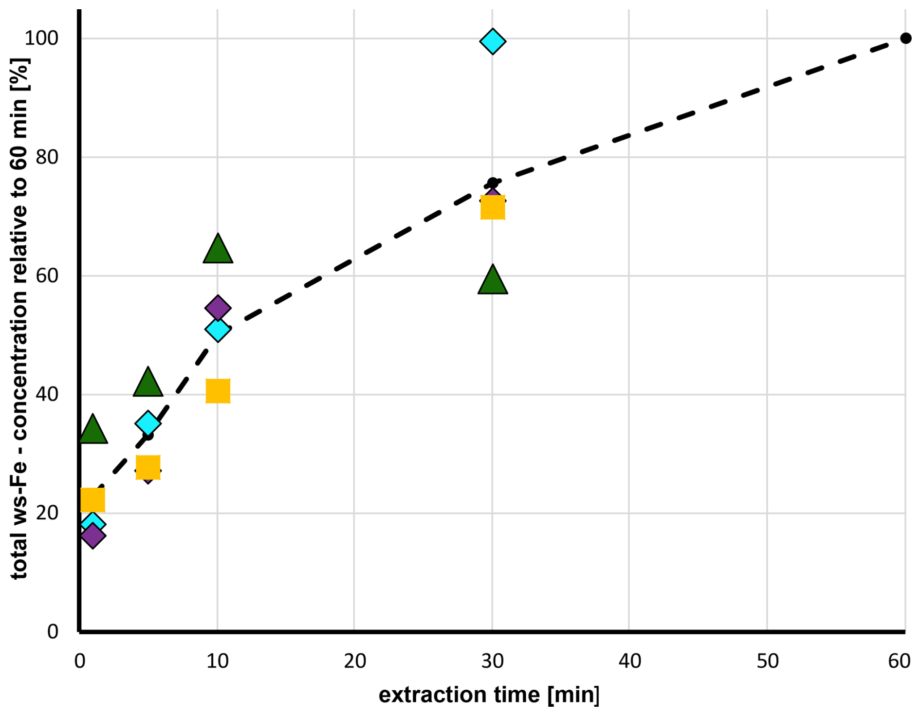
Figure 3 Total ws-Fe concentration relative to the total ws-Fe (II) concentration after 60 min as a function of extraction time for four filters (B5–B8) from the second field campaign. The filters were extracted in pH 4.5 solution and total ws-Fe was determined. Coloured symbols represent the efficiencies determined for the four different filter samples (B5–B8); the dashed black line indicates the average.

Overall, these results show that the extraction time is an important factor when determining the concentration of water-soluble iron at a cloud-water-relevant pH. As the extraction time in the online instruments is shorter compared to filter analysis, the concentration determined online might not represent the total extractable water-soluble-iron fraction. Therefore, extraction time is an important factor to consider when comparing measurements and interpretations between different studies.

3.2 Test campaigns and first field application

Concentrations of ws-Fe(II) and total ws-Fe were measured with both the online system and with offline filter samples during two test campaigns in Berlin: at Straße des 17. Juni in June 2024 and on the main campus of TU Berlin in March 2025.

3.2.1 Comparison of online and offline measurements

The concentrations of ws-Fe(II) (light red) and total ws-Fe (dark red) measured online during the two test campaigns are shown in Fig. 4. Shaded areas indicate values obtained from offline filter analysis. During the first campaign at Straße des 17. Juni in June 2024, online ws-Fe(II) and total ws-Fe concentrations varied between 1 and 9 ng m⁻³, except between 8 and 9 June 2024, when total ws-Fe reached 50 ng m⁻³ (Fig. 4a). On average, during the period the total online ws-Fe concentration was 5.2 ng m⁻³. Elevated water-soluble-iron concentrations during this period of the first campaign were also observed in the offline filter samples, with an average offline ws-Fe(II) concentration of 17.0 ng m⁻³ on 8 June 2024 (Table 3, filter A4). Averaged online ws-Fe(II) concentrations from the MARS-FIA system for the corresponding period were 19.5 ng m⁻³.

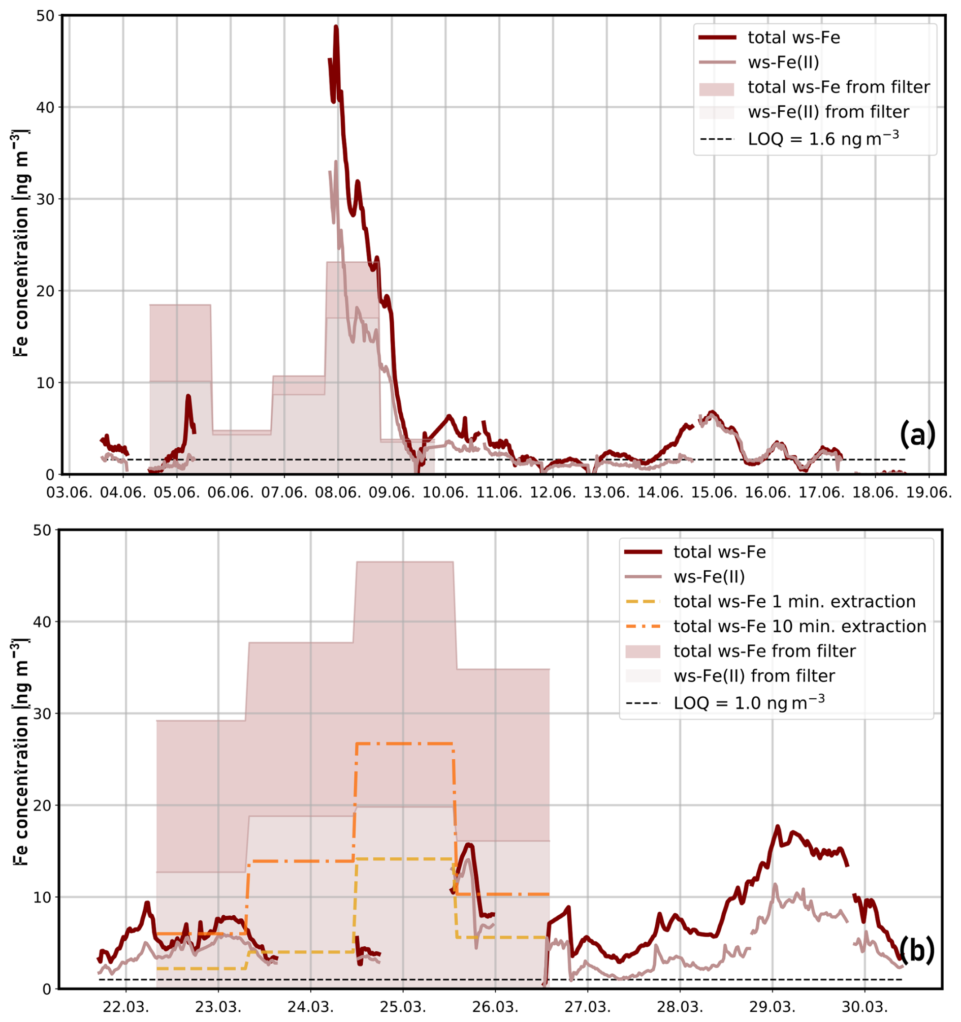
Figure 4 Temporal variability of total ws-Fe (red) and ws-Fe(II) (light red) concentrations in particulate matter (PM_2.5) in Berlin: (a) first test campaign with MARS-FIA setup at the road Straße des 17. Juni from 3 to 19 June 2024. The shaded areas represent the concentrations obtained by filter analysis with filter extraction in Seradest water. The dashed black line represents the LOQ from blank measurements. (b) Second test campaign with PILS-FIA setup at TU Berlin Campus from 22 to 30 March 2025. The shaded areas represent the concentrations obtained by filter analysis with extraction at pH 4.5. The dashed yellow line represents the concentrations from 1 min filter extraction at pH 4.5. The dashed orange line represents the concentrations after 10 min filter extraction at pH 4.5. The dashed black line represents the LOQ from blank measurements.

Table 3 Offline ws-Fe(II) and total ws-Fe concentrations from filter extraction. Filters were extracted for 1 h in pure Seradest water of pH 6.5 and with Seradest water adjusted to pH 4.5.

n.a.: no data available.

On 9 June 2024, ws-Fe(II) concentrations decreased rapidly to values below the limit of quantification. Filter-based ws-Fe(II) was 2.4 ng m⁻³ (Table 3, filter A5), while the online MARS-FIA system measured an average of 5.0 ng m⁻³. These results demonstrate a good agreement between online and offline measurements. The total ws-Fe concentrations for 8 and 9 June 2024, determined from filter analysis, were 23.1 and 3.1 ng m⁻³, respectively (Table 3, filters A4 and A5), while average total ws-Fe concentrations from the online MARS-FIA system were higher, i.e. 31.7 and 7.6 ng m⁻³, respectively. The total ws-Fe concentrations measured by MARS-FIA are thus substantially higher compared to the filter analysis. Both, dissolved Fe(II) and Fe(III) ions are not stable in water at pH 6.5. On the one hand, dissolved Fe(II) quickly oxidizes to Fe(III). Pham and Waite (2008) found a half-life time for the oxidation of 50 nM dissolved Fe(II) of approximately 5 h at pH 6, which increases with increasing pH. Furthermore, dissolved Fe(III) rapidly hydrolyses to form Fe(OH)²⁺ and can subsequently undergo further hydrolysis and precipitation. Extraction for 1 h in Seradest water at pH 6.5 may therefore result in both oxidation of dissolved Fe(II) and hydrolysis and precipitation of Fe(III). Potentially, this could result in an insufficient reduction time of HA in the FIA system to fully reduce already hydrolysed Fe(III) back to Fe(II) as it was observed with aged-Fe(III) standards (see Sect. 3.1.1), leading to lower measured total ws-Fe concentrations compared to the online MARS-FIA system, where the sample is analysed within minutes and, therefore, where less oxidation, hydrolysis, and precipitation can be expected.

The temporal variability of ws-Fe(II) and total ws-Fe concentrations during the field campaign with the PILS-FIA setup at the Campus of TU Berlin is illustrated in Fig. 4b. The concentration of total ws-Fe ranges between 1.0 and 17.7 ng m⁻³ and is thus not higher compared to the first field campaign even though the sample flow of the PILS-FIA setup was acidified to pH 4.5 (see Sect. 2.2.1). In the period of 22 to 26 March 2025, 24 h filters were collected (Table 3, filters B5–B8). To match the pH of extraction solution and wash flow from PILS, the filters were extracted at pH 4.5 with different extraction times (see Sect. 2.4.2). The shaded areas represent the concentrations determined for 1 h extraction time at pH 4.5. As highlighted in Fig. 4b, the concentrations determined for both ws-Fe(II) and total ws-determined are more than twice as high as those determined by the online PILS-FIA. A comparison of the concentration measured by PILS-FIA with those from the filters extracted for 1 min (dashed yellow line) and 10 min (dashed orange line, Fig. 4b) shows that 1 min extraction concentrations are lower than the online concentrations, while those after 10 min extraction fit well with concentrations determined with the online PILS-FIA setup. Due to missing PILS-FIA data from the evening of 24 March 2025 until the morning of 26 March 2025, only two filters (B5 and B8) can be compared with the online concentrations. The average concentrations determined with the PILS-FIA during the sampling period of filter B5 and B8 were 6.0 and 10.6 ng m⁻³, respectively. When comparing these concentrations with the concentrations after 1, 5, 10, and 30 min of extraction (Table A2), the concentrations after 10 min of extraction, i.e. 6.0 and 13.9 ng m⁻³, respectively, show very good agreement with the PILS-FIA measurement where the total residence time of the sample is around 15 min and 30 s (see Sect. 3.1.2).

The ratio between ws-Fe(II) and total ws-Fe of the online system in relation to the total ws-Fe concentrations of > 5 ng m⁻³ is shown in Fig. 5. Total ws-Fe concentrations of > 5 ng m⁻³ were chosen due to an increased relative error when calculating the ratios for lower total ws-Fe and ws-Fe(II) concentrations. The ratios during the summer test campaign with the MARS-FIA vary between mostly 0.5 and 0.7, resulting in an arithmetic mean of 0.66 and a median of 0.62 (Fig. 5a).

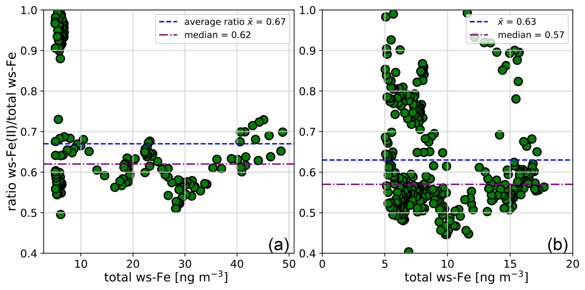
Figure 5 Ratios of ws-Fe(II) $/$ total ws-Fe concentration over total ws-Fe concentration of > 5 ng m⁻³ during (a) the MARS field test campaign at Straße des 17. Juni in June 2024 and (b) the PILS field test campaign on the campus of TU Berlin in March 2025.

The ratios during the winter test campaign with the PILS-FIA show higher variability compared to the first MARS-FIA test campaign, ranging from 0.4 to 1.0, resulting in an arithmetic mean of 0.63 and a median of 0.57 (Fig. 5b). The ratio of ws-Fe(II) to total ws-Fe of the filter samples is listed in Table 3. The ratios from filter analysis from the MARS-FIA vary between 0.55 and 0.81, resulting in an arithmetic mean of 0.69, thus being slightly higher compared to the ratios determined with the online system. The ratios of higher ws-Fe(II) to total ws-Fe from the filter samples compared to the ratio determined by MARS-FIA again reflect lower concentrations of total ws-Fe in offline filter analysis compared to the online system, as discussed above.

The arithmetic mean of the ratios of the four filters from the PILS-FIA test campaign, which were extracted at pH 4.5 for 1 h, is 0.82 and thus is significantly higher compared to the mean ratio determined from the PILS-FIA online concentrations, which is 0.63 and thus is similar to the first test campaign (MARS-FIA with Seradest extraction). While the ratios between the first and second field campaigns determined online were similar, even though they were conducted at different extraction pH levels, the ratios of ws-Fe(II) $/$ total ws-Fe from the filter extractions differ markedly between the two campaigns. The filter ratio from the first campaign (extracted with Seradest water at pH 6.5) is 0.61, while that from the second campaign (extracted at pH 4.5) is 0.82. This difference – comparable online ratios versus divergent offline ratios – highlights the influence of extraction time within the online system, which appears to have a higher impact than acidification of the sample flow.

In general, no temporal difference in the ratios observed during day and night could be identified (see Fig. A1). In a study by Majestic et al. (2006), filter samples from an urban station in St. Louis (August 2004) were extracted with different leachates, and the ws-Fe(II) and total ws-Fe concentrations were determined using the ferrozine method. In their study, ws-Fe concentrations ranged from 5 to 25 ng m⁻³, depending on the leachate used, resulting in ratios of ws-Fe(II) to total ws-Fe of 0.5 to 0.6. The ws-Fe(II) and total ws-Fe concentrations determined by both the MARS-FIA and PILS-FIA setups in this study are therefore consistent with previous work on ws-Fe in urban environments.

3.2.2 Comparison of ws-Fe With PM_2.5 and black carbon (BC)

During the first field campaign in June 2024, the MARS-FIA setup was placed close to the main artery road Straße des 17. Juni in the city centre of Berlin, thus measuring air which is highly influenced by traffic. Particle size distributions and BC concentrations were also measured (see Sect. 2.4.1). The temporal variability of PM_2.5 (light blue) and total ws-Fe (dark red) is illustrated in Fig. 6a. The PM_2.5 concentrations varied between 2 and 47 µg m⁻³, resulting in an average of 14 µg m⁻³. The total ws-Fe concentrations were 3 orders of magnitude lower, following the trend of the PM_2.5 concentrations. Between 7 and 8 June 2024, the PM_2.5 concentration remained relatively high around 30 µg m⁻³. Data for 7 June 2024 are missing from the PILS-FIA system, but the highest total ws-Fe concentrations measured during the period were between 40 and 50 ng m⁻³ on 8 June 2024, reaching a maximum of 48.7 ng m⁻³ when PM_2.5 concentrations were also high.

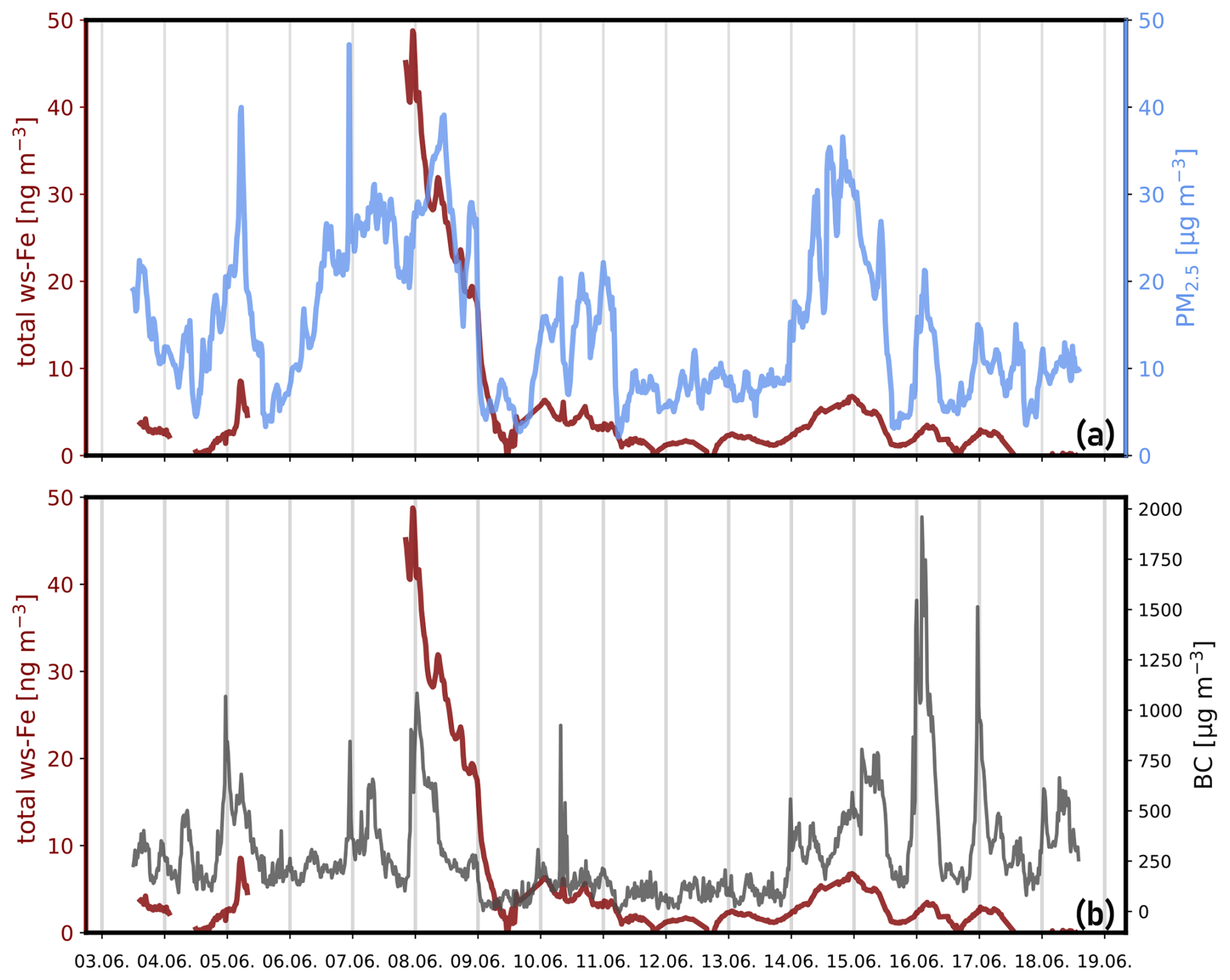
Figure 6 Temporal variability of total ws-Fe and PM_2.5 (a) and total ws-Fe and BC (b) during the first test campaign at Straße des 17. Juni in June 2024.

On the night of 9 June 2024, both concentrations dropped rapidly before they increased again on 10 June 2024. On 14 June 2024, PM_2.5 once again reached concentrations close to 40 µg m⁻³. Total ws-Fe concentrations also increased during that time, reaching a maximum of 6.8 ng m⁻³ at 23:20 CET on 14 June 2024. For the linear regression between PM_2.5 and total ws-Fe concentrations, a Pearson correlation coefficient of 0.49 indicates a moderate correlation (p < 3.4 × 10⁻⁴⁷). Plotting the PM_2.5 concentration against the total ws-Fe concentration (Fig. 7a), two distinct groups of data points appear to form. The total ws-Fe concentrations higher than 15 ng m⁻³, measured on 8 June 2024 and highlighted in beige in Fig. 7a, stand apart from the total ws-Fe concentrations below 15 ng m⁻³ from the rest of the campaign, shown in a brown colour. Focusing on the lower total ws-Fe concentrations (< 15 ng m⁻³) in Fig. 7b, these values correspond to a mass fraction of total ws-Fe between 0.15 ‰ and 2 ‰ of PM_2.5, with most mass fractions falling between 0.15 ‰ and 0.3 ‰. Contrarily to the low total ws-Fe concentrations, the high total ws-Fe concentrations (> 15 ng m⁻³) converge at a mass fraction of 2 ‰ of PM_2.5.

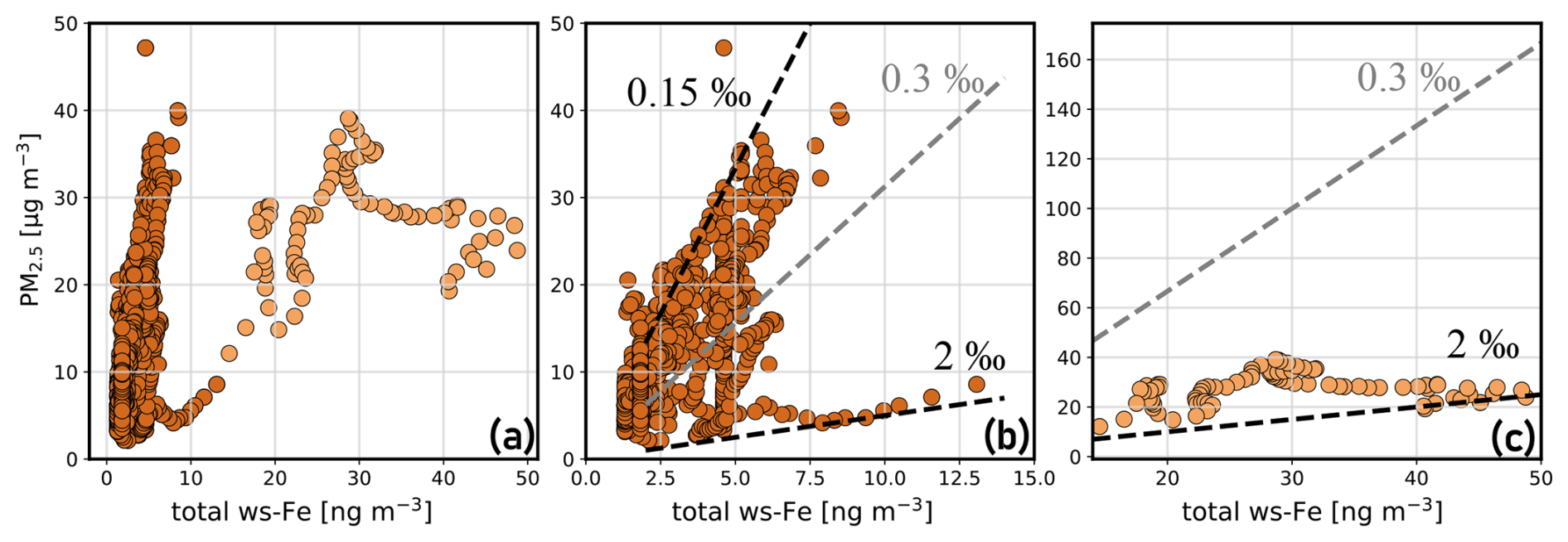
Figure 7 Relationship between PM_2.5 concentration and total ws-Fe concentration from the MARS-FIA test campaign in June 2024. (a) Scatterplot of all data points. PM_2.5 concentrations where the corresponding total ws-Fe concentration is < 15 ng m⁻³ are shown in brown. Those where total ws-Fe is > 15 ng m⁻³ are presented in beige. (b) Scatterplot of PM_2.5 versus total ws-Fe concentration of < 15 ng m⁻³. The dashed lines correspond to Fe mass fractions of 2 ‰, 0.3 ‰, and 0.15 ‰, illustrating the range of mass fractions of ws-Fe in PM_2.5 observed during the campaign. (c) Scatterplot of PM_2.5 versus total ws-Fe concentration > 15 ng m⁻³, illustrating that the mass fraction of total ws-Fe in PM_2.5 tends towards 2 ‰ for these concentration levels. Note the different scales in panel (c).

Salazar et al. (2020a) reported an average water-soluble-iron concentration of 7.7 ng m⁻³ in downtown Denver aerosols sampled during both summer and winter, corresponding to an average water-soluble-iron fraction of approximately 4.2 % of total iron. Crazzolara and Held (2024) measured a contribution of total iron in PM₁₀ ranging from 1.4 % to 3.7 % during a 1 d measurement campaign in the city centre of Berlin. Assuming a total iron content of 1 %–4 % in PM_2.5 and an iron solubility of 3 %–5 %, the expected total ws-Fe concentration would range from approximately 0.3 ‰ to 2 ‰ of the total PM_2.5 mass. This is consistent with our measurements and is evidence of the plausibility of the data. The elevated concentrations on 8 June 2024 may either reflect generally high total iron levels or indicate an emission event specifically rich in water-soluble iron.

The ratio between ws-Fe(II) and total ws-Fe on 8 June 2024 was 0.59, which is slightly lower compared to the arithmetic mean value of 0.67 in the campaign, indicating increased emissions of reducible Fe(III) compared to ws-Fe(II) on 8 June 2024.

The temporal variability of BC (grey) and total ws-Fe concentrations is illustrated in Fig. 6b. The concentration of BC varies between LOD and 2 µg m⁻³, reaching its maximum on 16 June 2024. For the linear regression between BC and total ws-Fe concentrations, a Pearson correlation coefficient of 0.35 (p < 1.87 × 10⁻²³) indicates a weaker correlation for BC compared to the PM_2.5 concentrations. On 8 June 2024, when total ws-Fe concentrations were high (> 15 ng m⁻³), BC concentrations were also elevated (see Fig. A2), indicating an emission event that could be connected to combustion processes such as traffic. ws-Fe concentrations originating from vehicle exhausts were investigated by Salazar et al. (2020b). They demonstrated that ws-Fe is formed through the dissolution of iron in water, mediated by specific organic compounds present in the exhaust. The authors proposed that anthropogenic ws-Fe mainly results from chelation with these organic compounds or their likely aqueous reaction products. In addition to organic compounds emitted directly from exhausts, common atmospheric ligands can enhance solubility, even under moderately acidic conditions (Chen and Grassian, 2013). Deprotonated ligands replace surface OH groups, thus forming a bidentate surface complex, which destabilizes the Fe–O bond (Wang et al., 2017). The formation of organic ligand–Fe complexes in the aqueous phase enhances further Fe dissolution from the aerosol into the liquid-water phase (Sakata et al., 2022). Oxalate, which is ubiquitously present in aerosol particles, is considered to be an important complexing ligand alongside formate and acetate. Recently, oxalate has been observed in aged dust particles, which can enhance dissolution (Li et al., 2025). The complexation of Fe(III) by such ligands can additionally promote the photo-reduction to Fe(II) (Shi et al., 2012). Increased solubility in fog samples in the presence of metal–organic complexes has, for example, been observed by Giorio et al. (2025).

The second field campaign was conducted in March 2025 on the TU Berlin campus with the PILS-FIA setup with a sample flow pH of 4.5. During this period, air quality in Berlin ranged from moderate to poor, as indicated by PM_2.5 concentrations at the Berlin background stations, which reached up to 40 µg m⁻³ and averaged 20 µg m⁻³ over 9 d (see Fig. A3). In contrast, the average PM_2.5 concentration during the first field campaign was only 8 µg m⁻³. The mean total ws-Fe concentration was 7.0 ng m⁻³, marginally higher than in the first campaign. Additionally, the variability in total ws-Fe concentrations was lower than previously observed, ranging from 2.7 to 17.2 ng m⁻³. The temporal patterns of both total ws-Fe (dark red) and PM_2.5 (light blue), as well as the total ws-Fe and black carbon (BC) concentrations (grey), are shown in Fig. A4. As in the first field campaign, total ws-Fe trends followed both the PM_2.5 and BC concentrations. The ratio of total ws-Fe to PM_2.5 was consistent with the first campaign, ranging between 0.15 ‰ and 2 ‰ (see Fig. A4a). The Pearson correlation coefficient between total ws-Fe concentrations of > 5 ng m⁻³ and PM_2.5 was 0.25 (p < 0.004), indicating a weak correlation. Similarly, a weak correlation was observed between total ws-Fe concentrations of > 5 ng m⁻³ and BC concentrations of < 800 µg m⁻³ (Pearson r = 0.28, p < 1.6 × 10⁵). The average ratio of ws-Fe(II) to total ws-Fe for concentrations above 5 ng m⁻³ was 0.63, only slightly lower than in the first campaign (see Fig. 5).

Overall, the second campaign, conducted in winter 2025 at the campus of TU Berlin, showed total ws-Fe concentrations that were comparable to those of the first campaign in summer (June 2024 at Straße des 17. Juni), thus indicating no clear seasonal difference even though the PM_2.5 concentrations of the background stations were notably higher during the winter test campaign. Salazar et al. (2020a) investigated ws-Fe concentrations at three locations, which were defined as (1) urban, (2) rural and agriculture, and (3) urban and agriculture in the summer and winter of 2016 and 2017. Across all three sites, they observed that ws-Fe concentrations were lower in winter, even though total iron concentrations were higher during that season. Similarly, Ye et al. (2018) analysed long-term filter samples collected in Atlanta from 1998 to 2013 and found that seasonal and long-term trends in ws-Fe closely followed sulfate concentrations, which were elevated in summer and showed a long-term decline attributed to reduced coal combustion. Based on the same data set, Wong et al. (2020) further concluded that sulfate promotes acidic aerosol conditions and particle water contents that enhance the dissolution of iron, with ws-Fe variability mainly being controlled by particle liquid water and stronger effects in summer, while combustion sources contribute relatively more in winter.

In Europe, sulfate concentrations decreased by approximately 0.15 µg yr⁻¹ between 2000 and 2018 (Tsimpidi et al., 2025). This long-term decline likely contributes to the generally lower ws-Fe concentrations observed during the Berlin campaigns compared to those reported for Atlanta between 2008 and 2013 (average of 24.22 ng m⁻³; Ye et al., 2018). Nevertheless, ws-Fe concentrations measured during 1 week in March 2025 and during nearly 3 weeks in June 2025 were comparable despite representing different seasons.

The absence of a clear seasonal difference in the present study may partly result from comparing measurements at two nearby sites that are differently influenced by traffic. Importantly, however, the results of the second test campaign underline that the slightly acidic wash flow of pH 4.5 used in the PILS-FIA setup does not significantly affect iron's solubility or oxidation state during sampling compared to sampling using MARS with pH 6.5.

4 Suitability of the FIA system for field measurements

Both field test campaigns demonstrate that the developed FIA system, designed for near-real-time measurement of ws-Fe(II) and total ws-Fe concentrations in particulate matter, can be effectively used in combination with the MARS and PILS sampling units in an urban environment. The system is suitable for urban environments where total ws-Fe concentrations exceed 1 ng m⁻³. To assess its applicability under different environmental conditions, filter samples were collected at Mace Head, Ireland, as described in Sect. 2.3.2. Because Mace Head represents a pristine environment with expectedly low iron concentrations, filter sampling with sampling periods between 5 and 10 d was performed. Results shown in Table 3 indicate very low total ws-Fe concentrations – ranging from < LOQ to 0.05 ng m⁻³ – when extracted with Seradest water at pH 6.5. These findings illustrate the substantially lower iron solubility in regions with minimal anthropogenic emissions. Even after acidifying the extraction solution to pH 4.5, representing cloud-water-relevant conditions, total ws-Fe concentrations ranged between 0.13–0.29 ng m⁻³, thus still remaining below 1 ng m⁻³.

For application at remote sites with total ws-Fe concentrations below 1 ng m⁻³, the LOQs of both the MARS-FIA and PILS-FIA setups, given their current settings, are too high to reliably detect near-real-time ws-Fe concentrations. Further acidification of the wash flow to pH 2 or 3 is unlikely to sufficiently boost water-soluble-iron concentrations due to the short extraction times available. Therefore, quantification of ws-Fe in remote locations would require methodological adaptations, such as pre-concentration, increasing the extraction time within the sampling unit, extending the residence time in the online apparatus before ferrozine addition, or increasing the ratio of gas volume to volume of extractant by collecting larger air sample volumes. Nevertheless, the FIA system was successfully applied in two field campaigns in Berlin and provides the speciation capability of water-soluble iron in ambient aerosols in future field measurements, especially in urban and semi-urban environments.

Appendix A

Table A1 Results of linear regression from calibration over 1 year.

Table A2 Total ws-Fe concentration depending on the extraction time in acidified water (pH 4.5).

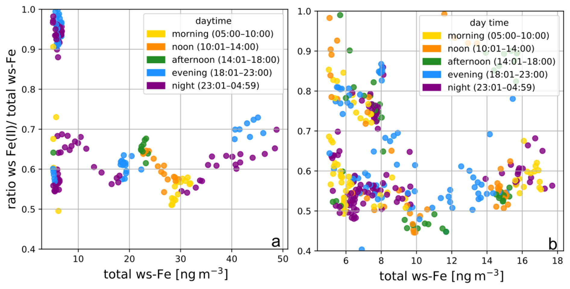
Figure A1 Ratios of ws-Fe(II) to total ws-Fe over total ws-Fe concentration of > 5 ng m⁻³, coloured depending on the time of the day (a) at Straße des 17. Juni and (b) on the campus of TU Berlin.

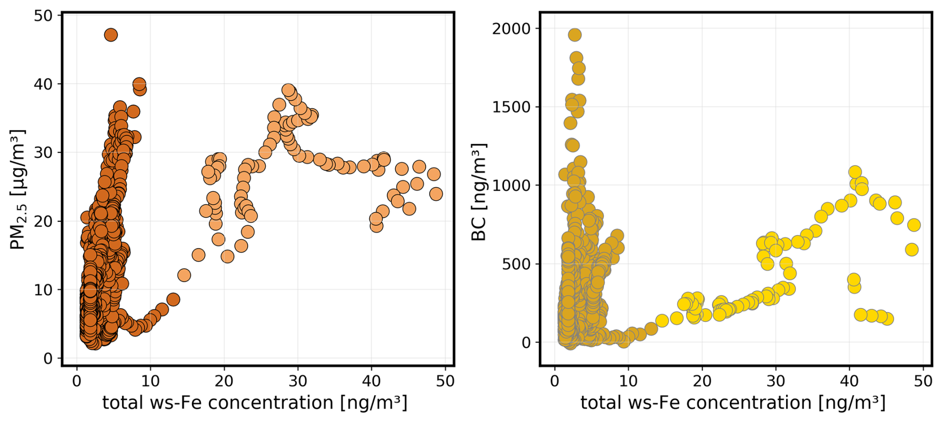
Figure A2 Total ws-Fe concentration to PM_2.5 concentrations (left) and BC concentrations (right).

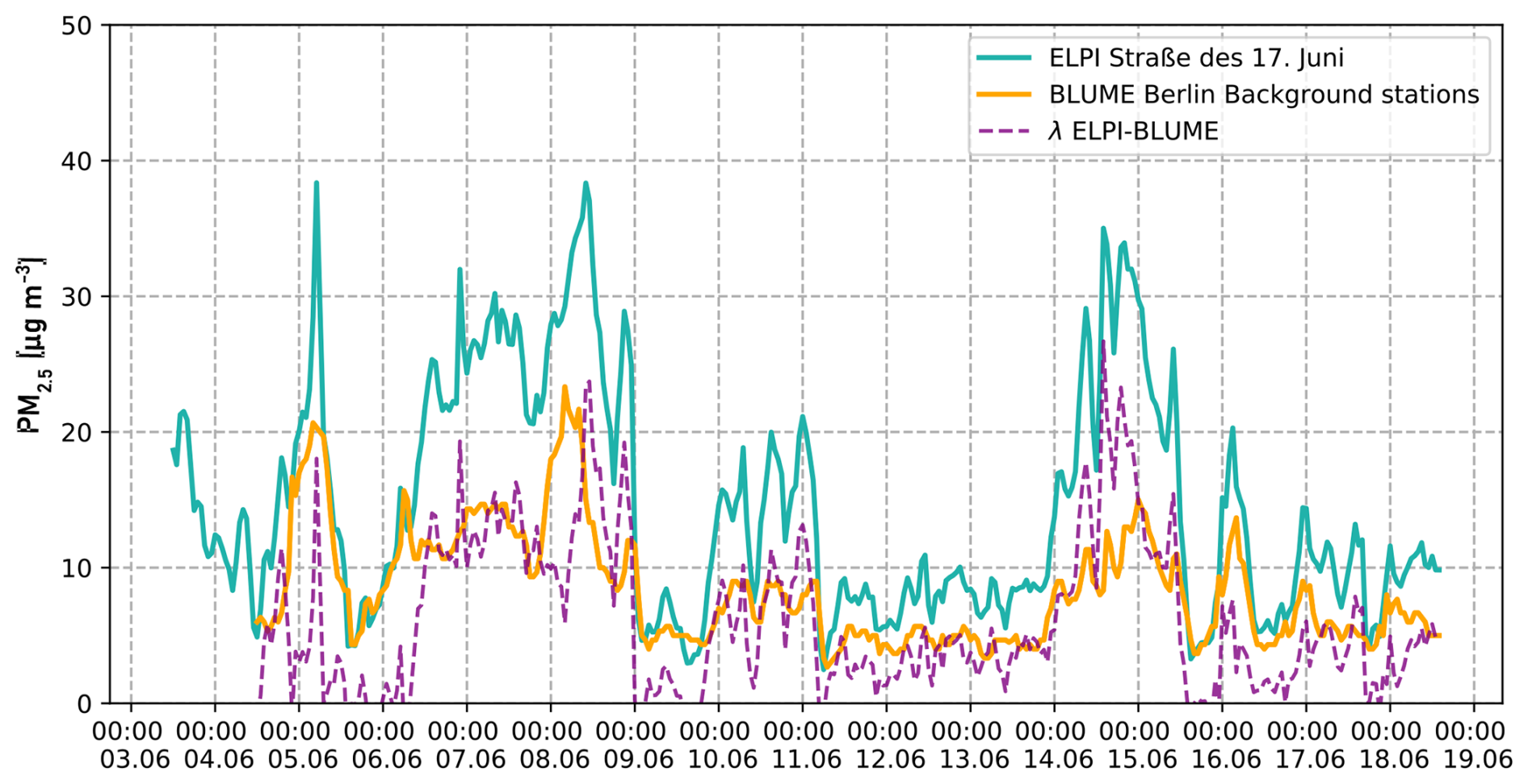
Figure A3 Temporal variability of PM_2.5 concentrations at Straße des 17. Juni (turquoise) and average concentrations from background stations Neukölln, Mitte, and Wedding from the Berlin BLUME air quality network (yellow). The dashed purple lines represent the difference between the ELPI measurements at Straße des 17. Juni and the averaged concentrations from the BLUME air quality network.

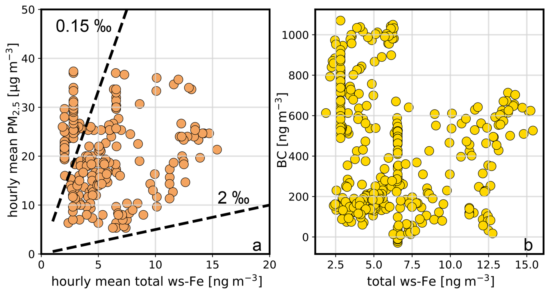
Figure A4 Hourly averaged PM_2.5 concentration from BLUME background stations over hourly averaged total ws-Fe concentration (a) and BC concentration over total ws-Fe concentrations (b).