The Centrifugal Differential Mobility Analyser – concept and initial validation of a new device for measuring 2D property distributions

Usually for the characterization of nanoparticles, an equivalent property is measured, e.g. the mobility-equivalent diameter. In the case of non-spherical, complex-shaped nanoparticles, one equivalent particle size is not sufficient for a complete characterization. Most of the methods utilized to gain deeper insight into the morphology of nanoparticles are very time-consuming and costly or have bad statistics (such as tandem setups or TEM (transmission electron microscopy)/SEM (scanning electron microscopy) images). To overcome these disadvantages, a prototype of a new compact device, the Centrifugal Differential Mobility Analyser (CDMA), was built, which can measure the full 2D distribution of mobility-equivalent and Stokes equivalent diameters by classification in a cylinder gap through electrical and centrifugal forces. An evaluation method to determine the transfer probabilities is developed and used in this work to compare the measurement results with the theory for the pure rotational behaviour (like the Aerodynamic Aerosol Classifier) and the pure electrical behaviour (like the Dynamic Mobility Analyser). In addition, the ideal 2D transfer function was derived using a particle trajectory approach. This 2D transfer function is a prerequisite for obtaining the full 2D particle size distribution from measurements by inversion.

1 Introduction

A common feature of many techniques is that, for non-spherical particles, they measure an equivalent particle size. For example, the Differential Mobility Analyser (DMA) (Knutson and Whitby, 1975) measures the mobility-equivalent diameter. The Aerodynamic Aerosol Classifier (AAC) (Tavakoli and Olfert, 2013), the Low Pressure Impactor (LPI) (Fernandez de la Mora et al., 1989), and the Aerodynamic Particle Sizer (APS) (Mitchell et al., 2003) measure the aerodynamic-equivalent diameter. The Centrifugal Particle Mass Analyser (CPMA) (Olfert and Collings, 2005) measures the mass–charge ratio. However, this information alone is not sufficient to determine the actual particle properties comprehensively, especially in the case of large agglomerates, which may have significantly different shapes than spherical particles. Therefore, numerous studies have focused on this topic. In particular, the influence of particle shape on bio-availability and toxicity (Jindal, 2017; Toy et al., 2014) as well as on environmental aerosols is a topic of great scientific interest (Kelesidis et al., 2022). The effects of particle shape on the mechanical stability and reaction rates of batteries have also been investigated (Zhang et al., 2022). Due to its relevance, many research institutions are focusing on separation by more than one particle property to produce highly specific particle systems (Rhein et al., 2019; Sandmann and Fritsching, 2023; Furat et al., 2020, 2019).

In order to design and control these processes effectively, it is essential to develop techniques to assess the particle structure and dimensions. Scanning electron microscopy (SEM) studies at least offer full shape information in 2D for this purpose, but imaging the full particle size distribution requires a significant number of images, which can be both time-consuming and costly. An alternative approach is tandem setups, i.e. a serial arrangement of two different classification systems, allowing the determination of two different equivalent particle sizes. This can provide more comprehensive information and can be used to derive enhanced, more specific structure information, e.g. the effective density or fractal dimension (Park et al., 2008; Slowik et al., 2004; Tavakoli and Olfert, 2013).

The CDMA (Centrifugal Differential Mobility Analyser) is a recently developed compact device that has been designed to address the limitations of existing tandem setups, particularly the high costs of equipment and the complexity of the associated measurement procedures. Furthermore, the measurement and evaluation can be conducted directly with the CDMA, which significantly reduces the analytical burden and the user's required knowledge for calculating such measurements.

The objective is to obtain a complete 2D particle size distribution expressed in terms of the Stokes equivalent and mobility-equivalent diameters. The combination of these two properties allows us to draw conclusions about the particle geometry. That is, a complete 2D property distribution of the effective density or fractal dimension can be calculated, thus facilitating an even more precise and comprehensive investigation of the distribution shape. Additionally, the large number of examined particles enhances the statistical reliability of the findings, exceeding SEM examinations. Furthermore, additional examinations can be conducted using this approach. For example, it may be possible to measure the charge distribution of specific particles or to investigate the influence of particle shape on charge distribution.

2 Concept and fundamental theory

The newly developed principle of the CDMA combines the concepts of the DMA and AAC. In general, the CDMA consists of two concentric cylinders between which high voltage can be applied. Both of them can be rotated at the same angular speed. This means that both the voltage and the speed can be superimposed, whereas in the DMA only the voltage can be varied and, in the AAC, only the speed. This means that, with the CDMA, particles can be classified according to their drag force and mass. In the DMA particles are usually characterized by their mobility diameter d_m (i.e. the diameter of a spherical particle experiencing the same drag force for a given relative velocity as the actual particle) (Friedlander, 2000). The AAC typically uses the aerodynamic diameter d_ae to characterize particles (i.e. the diameter of a sphere with unit density and the same settling velocity), which has the advantage that all particles of the same settling velocity in the centrifugal field will have the same equivalent diameter (Tavakoli and Olfert, 2014). However, particles with exactly the same shape but a different material density will show different aerodynamic diameters. Since in our instrument the 2D characterization mainly aims to characterize the particle shape, we suggest using the Stokes diameter d_St instead (i.e. the diameter of a sphere of the same density with the same settling velocity w_S as the actual particle) for characterization (Colbeck, 2013; Reist, 1993). Although both equivalent sizes are closely related, the Stokes diameter only depends on the particle shape, e.g. characterized by the volume- and mobility-equivalent diameters d_v and d_m, respectively (Baron et al., 2011).

$$\begin{array}{}\text{(1)}& d_{\mathrm{St}}=\sqrt{{\displaystyle \frac{\mathrm{18}\mathit{\eta }}{{\mathit{\rho }}_{\mathrm{S}}\cdot b\cdot \mathrm{Cu}\left(d_{\mathrm{m}}\right)}}\cdot w_{\mathrm{s}}}=\sqrt{{\displaystyle \frac{{\mathit{\rho }}_{\mathrm{0}}}{{\mathit{\rho }}_{\mathrm{S}}}}}\cdot d_{\mathrm{ae}}=\sqrt{{\displaystyle \frac{d_{\mathrm{v}}^{\mathrm{3}}}{d_{\mathrm{m}}}}}\end{array}$$

η is the dynamic viscosity, ρ_S the solid density of the particle material, ρ₀ the unit density of 1000 kg m⁻³, b the centrifugal or gravitational acceleration, and w_S the settling velocity. In particular, the Stokes and mobility diameters become identical in the case of a perfect sphere. However, the calculation of the Stokes diameter from classification according to the settling velocity in the CDMA centrifugal field requires knowledge of the particle density. Therefore, if the density is not known with sufficient accuracy or an aerosol consisting of different materials is analysed, the aerodynamic diameter should be used as in classical AAC theory. This can easily be adapted in the inversion algorithm. However, if the density of the particles is unknown, the shape information will no longer be accessible. By measuring all voltage–speed combinations, a full 2D particle size distribution in terms of d_st and d_m can be calculated by data inversion.

When an aerosol volume flow Q_a is the inner cylinder, the particles are displaced by electrical forces and centrifugal forces which always drive the particles towards the outer cylinder (Fig. 1). Particles pass through the sheath airflow Q_sh and are classified and counted in the sample flow Q_s if they meet the specified characteristics.

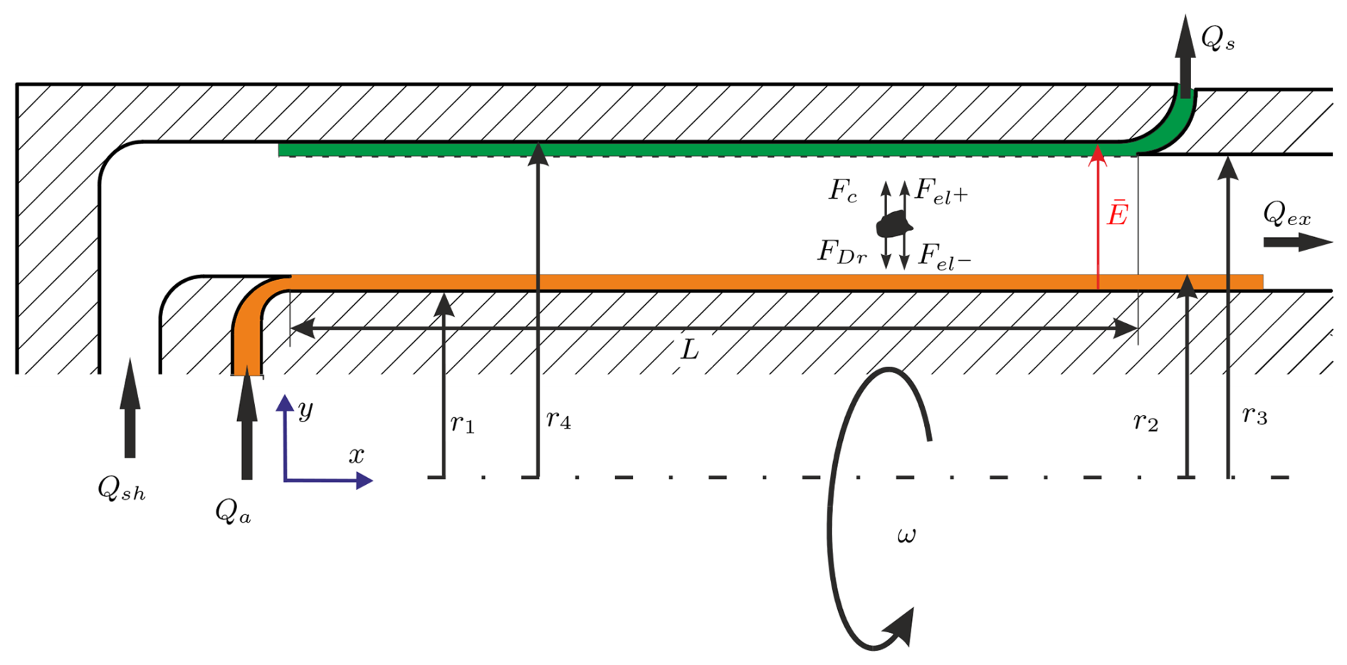
Figure 1 Schematic drawing of the classification zone of the CDMA: sheath air Q_sh, exhaust air Q_ex, sample air Q_s, aerosol air Q_a, electrical field magnitude E, rotational speed ω, electrical force F_el, centrifugal force F_c, drag force F_Dr, length of the transfer path L, inner radius r₁, maximum radius at which the particles enter r₂, minimum radius at which the particles are still classified r₃, and outer radius r₄.

Because inertial forces are typically negligible, the quasi-static particle drift velocity w_Dr can be obtained from a force balance. Assuming Stokes' drag then leads to

$$\begin{array}{}\text{(2)}& Q_{\mathrm{P}}\cdot E+m_{\mathrm{P}}\cdot a_{\mathrm{c}}=\mathrm{3}\mathit{\pi }\mathit{\eta }{d}_{\mathrm{m}}{w}_{\mathrm{Dr}}/\mathrm{Cu},\end{array}$$

with particle charge Q_P, electrical field magnitude E (as defined like in Fig. 1), particle mass m_P, centrifugal acceleration a_c=ω²r, dynamic viscosity η, mobility diameter d_m, particle drift velocity w_Dr, and Cunningham correction factor Cu (Allen and Raabe, 1985).

The limiting cases E=0 and ω=0 in Eq. (2) lead to the equations from the derivations of the DMA (Stolzenburg, 1988) and AAC (Tavakoli and Olfert, 2014), respectively.

Using the same assumptions as in the boundary cases – i.e. no diffusion, plug flow, and no perturbations of the E field (ideal geometry, no room charges, and no inertial forces) – the deterministic description of the particle's path is achieved by rearranging and integrating Eq. (2).

$$\begin{array}{}\text{(3)}& \begin{array}{rl}& r\left(y\right)=\\ & \sqrt{{\displaystyle \frac{\left(\mathit{\tau }\cdot {\mathit{\omega }}^{\mathrm{2}}\cdot r_{\mathrm{in}}^{\mathrm{2}}+\frac{Z\cdot U}{\ln \left(\frac{r_{\mathrm{4}}}{r_{\mathrm{1}}}\right)}\right)\cdot \exp \left\{\mathrm{2}\cdot \mathit{\tau }\cdot {\mathit{\omega }}^{\mathrm{2}}\cdot y\cdot \frac{\mathit{\pi }\cdot \left(r_{\mathrm{4}}^{\mathrm{2}}-r_{\mathrm{1}}^{\mathrm{2}}\right)}{Q_{\mathrm{sh}}+Q_{\mathrm{a}}}\right\}-\frac{Z\cdot U}{\ln \left(\frac{r_{\mathrm{4}}}{r_{\mathrm{1}}}\right)}}{\mathit{\tau }\cdot {\mathit{\omega }}^{\mathrm{2}}}}},\end{array}\end{array}$$

with the voltage U, the rotational velocity ω, the inner r₁ and outer r₄ radii, the actual radius at which the particle enters r_in, the length of the classifying gap L, the position of the particle in the streamwise direction y, the particle relaxation time τ (Tavakoli and Olfert, 2014)¹, and the particle mobility Z (Stolzenburg, 1988).

$$\begin{array}{}\text{(4)}& \mathit{\tau }={\displaystyle \frac{\mathit{\rho }\cdot d_{\mathrm{v}}^{\mathrm{3}}\cdot \mathrm{Cu}\left(d_{\mathrm{m}}\right)}{\mathrm{18}\cdot d_{\mathrm{m}}\cdot \mathit{\eta }}}={\displaystyle \frac{\mathit{\rho }\cdot d_{\mathrm{st}}^{\mathrm{2}}\cdot \mathrm{Cu}\left(d_{\mathrm{m}}\right)}{\mathrm{18}\mathit{\eta }}},\end{array}$$

$$\begin{array}{}\text{(5)}& Z={\displaystyle \frac{n\cdot e\cdot \mathrm{Cu}\left(d_{\mathrm{m}}\right)}{\mathrm{3}\mathit{\pi }\cdot \mathit{\eta }\cdot d_{\mathrm{m}}}},\end{array}$$

where ρ is the particle density, d_st is the Stokes equivalent diameter, d_v is the volume-equivalent diameter, n is the number of charges carried by a particle, e is the elementary charge, and Q_ex is the exhaust gas volume flow.

The dimensionless, normalized mobility or particle relaxation time is obtained as follows:

$$\begin{array}{}\text{(6)}& \stackrel{\mathrm{̃}}{Z}=Z/Z^{\ast };\stackrel{\mathrm{̃}}{\mathit{\tau }}=\mathit{\tau }/{\mathit{\tau }}^{\ast },\end{array}$$

where Z^∗ is the mobility required for a particle entering at the centre of the aerosol inlet to be sampled at exactly the centre of the outlet (Stolzenburg, 1988). τ^∗ describes the same behaviour but for the relaxation time (Tavakoli and Olfert, 2014).

$$\begin{array}{}\text{(7)}& Z^{\ast }={\displaystyle \frac{Q_{\mathrm{sh}}+Q_{\mathrm{ex}}}{\mathrm{4}\cdot \mathit{\pi }\cdot \mathrm{L}\cdot \mathrm{U}}}\cdot \ln \left({\displaystyle \frac{r_{\mathrm{4}}}{r_{\mathrm{1}}}}\right)\end{array}$$

$$\begin{array}{}\text{(8)}& {\mathit{\tau }}^{\ast }={\displaystyle \frac{Q_{\mathrm{sh}}+Q_{\mathrm{ex}}}{\mathit{\pi }{\mathit{\omega }}^{\mathrm{2}}(r_{\mathrm{1}}+r_{\mathrm{4}}{)}^{\mathrm{2}}L}}\end{array}$$

For typical operating conditions (Q_s=Q_a), a dimensionless form of Eq. (3) can be derived, where $\stackrel{\mathrm{‾}}{r}=\frac{r_{\mathrm{1}}+r_{\mathrm{4}}}{\mathrm{2}}$ is the average of the outer and inner radii, $\mathit{\beta }=\frac{Q_{\mathrm{a}}}{Q_{\mathrm{sh}}}$ is the ratio of the aerosol-to-sheath airflow, and $\stackrel{\mathrm{̃}}{h}=\frac{r_{\mathrm{4}}-r_{\mathrm{1}}}{\stackrel{\mathrm{‾}}{r}}$ is the ratio of the gap height to $\stackrel{\mathrm{‾}}{r}$.

$$\begin{array}{}\text{(9)}& r\left(y\right)=\sqrt{r_{\mathrm{in}}^{\mathrm{2}}\cdot \exp \left\{{\displaystyle \frac{y}{L}}\cdot \stackrel{\mathrm{̃}}{\mathit{\tau }}\cdot {\displaystyle \frac{\mathrm{2}\stackrel{\mathrm{̃}}{h}}{\mathrm{1}+\mathit{\beta }}}\right\}+{\stackrel{\mathrm{‾}}{r}}^{\mathrm{2}}\cdot {\displaystyle \frac{\stackrel{\mathrm{̃}}{Z}}{\stackrel{\mathrm{̃}}{\mathit{\tau }}}}\cdot \left[\exp \left\{{\displaystyle \frac{y}{L}}\cdot \stackrel{\mathrm{̃}}{\mathit{\tau }}\cdot {\displaystyle \frac{\mathrm{2}\stackrel{\mathrm{̃}}{h}}{\mathrm{1}+\mathit{\beta }}}\right\}-\mathrm{1}\right]}\end{array}$$

Figure 2 Cross section of the CDMA prototype.

3 CDMA prototype

To validate the functional principle, a prototype was designed and built. As a boundary condition, this prototype should be able to measure particle sizes ranging from 50 to 1000 nm for both the mobility-equivalent diameter and the Stokes equivalent diameter. In addition, the speed should not exceed 6000 rpm, because the ferrofluid sealing has only been tested in this range (with higher angular speeds, the sealing could evaporate much more quickly and produce particles itself) and to prevent unbalanced forces on the bearings.

3.1 Design

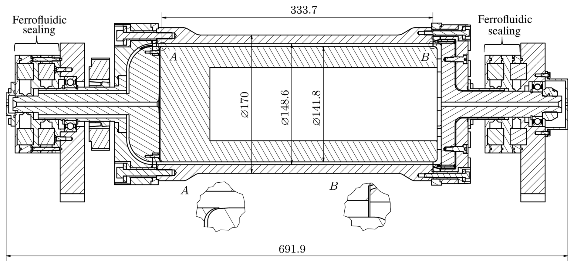
Figure 2 shows the cross section of the CDMA prototype and its dimensions.

At flow rates of Q_a=0.3 lpm and Q_sh=3 lpm, and assuming a particle density of 1000 kg m⁻³, these dimensions enable the characterization of particles in the size range from 50 to 1000 nm, where the maximum speed is 6000 rpm and the maximum voltage is limited to 1000 V².

One difficulty was in achieving a suitable seal against the environment. Friction seals are not an option, as either the sealing of the system is difficult or the seal heats up strongly due to high friction, generating particles, or abrasion occurs in general. Therefore, a ferrofluid seal was designed and tested. A ring magnet is used. On the outside of the ring magnet there are iron components that create a pole shoe on the inside of the ring. This pole shoe has a tolerance of approximately +0.1 mm of the shaft passing through it. The ferrofluid is injected into the pole shoe. This creates a virtually frictionless seal that does not generate particles.

The aerosol is fed into the long bore on the left, entering the classifying gap at point A. The sheath air is fed between the two ferrofluid sealings (this drilling is not visible in Fig. 2), entering the CDMA through eight axial holes and finally also the classifying gap via a bend. At the end of the classifying gap (point B), the sample flow is diverted outwards so that the particles are directed through narrow gaps towards the ferrofluid sealing and released at the centre of the seal. The sampled particles can then be counted by a CPC or similar instrument. The excess gas flow is sucked in towards the centre and directed through the long bore to the right, where it is purified for return to the inlet of the CDMA as the sheath airflow.

A toothed belt is used to transmit the forces of the motor to the rotating cylinder. A negative high potential is applied to the centre of the outer cylinder. This area is electrically isolated from the rest of the CDMA by insulators (outside between points A and B). The other components, like the inner electrode and all kinds of bearings, sealings, and housings, are connected to Earth so that there is mass potential, creating a voltage and thus an electrical field between the electrodes. This leads the electrical force of positively charged particles to be in the direction of the centrifugal force.

3.2 Particle losses

Particle losses occur due to the classification principle in the inlet and outlet areas of the CDMA. This occurs, in particular, during rotation, as the centrifugal force then acts on the particles in all the rotating feed and discharge pipes. This movement pushes the particles further towards the respective outer wall, where they are separated. Walls with a large radius running parallel to the axis of rotation are particularly susceptible because of the higher exerting centrifugal forces.

Separation can be calculated individually for each part. Dividing the radial distance s the particles move in each part by the distance between the walls s_max gives the degree of separation, assuming a laminar flow profile and a uniform concentration across the flow cross section³.

$$\begin{array}{}\text{(10)}& T=s/s_{\max }\end{array}$$

In addition, losses occur when the voltage is applied. Since a polymeric material (yellow regions in Fig. 3) was used to insulate the high-voltage outer electrode directly in the input and output regions, an electrical field is even generated in the input and output gaps due to the insulating properties of the air. Figure 3 shows a simulation with the Ansys Electronics software, which was used to simulate the field strengths at an applied voltage of 100 V. It can be seen that the field strength is partly as high as in the classifying gap. Hence, the simulation can also be used to calculate a theoretical deposition analogous to rotation.

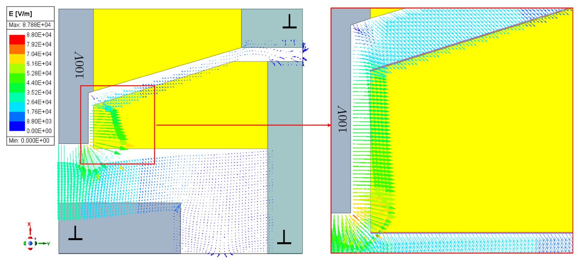
Figure 3 Electrostatic simulation of the outlet using Ansys Electronics at an applied voltage of 100 V.

4 The transfer function

The transfer function Ω describes the probability of a particle with certain properties (relaxation time τ and mobility Z) being successfully classified under given operating conditions (voltage U and angular velocity ω).

4.1 Two-dimensional transfer function based on the particle trajectory calculation

Since in CDMA, as in DMA and AAC, the ratio of aerosol volume flow to sheath air volume flow cannot be infinitely small and the inlet and sample gaps are also finite, the classified aerosol is not completely monomodal, but a distribution exists.

Assuming a constant particle flux density at the inlet, stratified plug flow, a homogeneous E field in the classifying gap, and non-inertial and diffusion-free particles, this distribution can be calculated analytically. The assumption of a plugflow profile is justified, since, for classifying a particle, the mean velocity is mainly relevant, since the particle path crosses the whole flow domain. Stolzenburg (1988) proved this with the derivation of transfer functions based on a streamline approach for diffusing particles. The derivation of the 2D transfer function is given in Appendix B.

Therefore, the transfer function Ω can be calculated as follows:

$$\begin{array}{}\text{(11)}& {\mathrm{\Omega }}_{\mathrm{CDMA}}=\max \left[\min \left(f_{\mathrm{1}},f_{\mathrm{2}},\mathrm{1}\right),\mathrm{0}\right],\end{array}$$

with

$$\begin{array}{}\text{(12)}& \begin{array}{rl}& f_{\mathrm{1}}={\displaystyle \frac{\frac{\mathit{\beta }+{\mathit{\kappa }}^{\mathrm{2}}}{\mathrm{1}+\mathit{\beta }}-(\frac{\mathrm{1}/\mathit{\beta }+{\mathit{\kappa }}^{\mathrm{2}}}{\mathrm{1}/\mathit{\beta }+\mathrm{1}}+\frac{(\mathit{\kappa }+\mathrm{1}{)}^{\mathrm{2}}}{\mathrm{4}}\cdot \frac{\stackrel{\mathrm{̃}}{Z}}{\stackrel{\mathrm{̃}}{\mathit{\tau }}})\cdot \exp \left\{-\stackrel{\mathrm{̃}}{\mathit{\tau }}\cdot \frac{\mathrm{2}\stackrel{\mathrm{̃}}{h}}{\mathrm{1}+\mathit{\beta }}\right\}+\frac{(\mathit{\kappa }+\mathrm{1}{)}^{\mathrm{2}}}{\mathrm{4}}\cdot \frac{\stackrel{\mathrm{̃}}{Z}}{\stackrel{\mathrm{̃}}{\mathit{\tau }}}}{\frac{\mathit{\beta }+{\mathit{\kappa }}^{\mathrm{2}}}{\mathrm{1}+\mathit{\beta }}-{\mathit{\kappa }}^{\mathrm{2}}}}-\\ & \max \left({\displaystyle \frac{\frac{\mathit{\beta }+{\mathit{\kappa }}^{\mathrm{2}}}{\mathrm{1}+\mathit{\beta }}-(\mathrm{1}+\frac{(\mathit{\kappa }+\mathrm{1}{)}^{\mathrm{2}}}{\mathrm{4}}\cdot \frac{\stackrel{\mathrm{̃}}{Z}}{\stackrel{\mathrm{̃}}{\mathit{\tau }}})\cdot \exp \left\{-\stackrel{\mathrm{̃}}{\mathit{\tau }}\cdot \frac{\mathrm{2}\stackrel{\mathrm{̃}}{h}}{\mathrm{1}+\mathit{\beta }}\right\}+\frac{(\mathit{\kappa }+\mathrm{1}{)}^{\mathrm{2}}}{\mathrm{4}}\cdot \frac{\stackrel{\mathrm{̃}}{Z}}{\stackrel{\mathrm{̃}}{\mathit{\tau }}}}{\frac{\mathit{\beta }+{\mathit{\kappa }}^{\mathrm{2}}}{\mathrm{1}+\mathit{\beta }}-{\mathit{\kappa }}^{\mathrm{2}}}},\mathrm{0}\right),\end{array}\end{array}$$

$$\begin{array}{}\text{(13)}& \begin{array}{rl}& f_{\mathrm{2}}={\displaystyle \frac{(\mathrm{1}+\frac{(\mathit{\kappa }+\mathrm{1}{)}^{\mathrm{2}}}{\mathrm{4}}\cdot \frac{\stackrel{\mathrm{̃}}{Z}}{\stackrel{\mathrm{̃}}{\mathit{\tau }}})\cdot \exp \left\{-\stackrel{\mathrm{̃}}{\mathit{\tau }}\cdot \frac{\mathrm{2}\stackrel{\mathrm{̃}}{h}}{\mathrm{1}+\mathit{\beta }}\right\}-\frac{(\mathit{\kappa }+\mathrm{1}{)}^{\mathrm{2}}}{\mathrm{4}}\cdot \frac{\stackrel{\mathrm{̃}}{Z}}{\stackrel{\mathrm{̃}}{\mathit{\tau }}}-{\mathit{\kappa }}^{\mathrm{2}}}{\frac{\mathit{\beta }+{\mathit{\kappa }}^{\mathrm{2}}}{\mathrm{1}+\mathit{\beta }}-{\mathit{\kappa }}^{\mathrm{2}}}}-\\ & \max \left({\displaystyle \frac{\left(\frac{\mathrm{1}/\mathit{\beta }+{\mathit{\kappa }}^{\mathrm{2}}}{\mathrm{1}/\mathit{\beta }+\mathrm{1}}+\frac{(\mathit{\kappa }+\mathrm{1}{)}^{\mathrm{2}}}{\mathrm{4}}\cdot \frac{\stackrel{\mathrm{̃}}{Z}}{\stackrel{\mathrm{̃}}{\mathit{\tau }}}\right)\cdot \exp \left\{-\stackrel{\mathrm{̃}}{\mathit{\tau }}\cdot \frac{\mathrm{2}\stackrel{\mathrm{̃}}{h}}{\mathrm{1}+\mathit{\beta }}\right\}-\frac{(\mathit{\kappa }+\mathrm{1}{)}^{\mathrm{2}}}{\mathrm{4}}\cdot \frac{\stackrel{\mathrm{̃}}{Z}}{\stackrel{\mathrm{̃}}{\mathit{\tau }}}-{\mathit{\kappa }}^{\mathrm{2}}}{\frac{\mathit{\beta }+{\mathit{\kappa }}^{\mathrm{2}}}{\mathrm{1}+\mathit{\beta }}-{\mathit{\kappa }}^{\mathrm{2}}}},\mathrm{0}\right),\end{array}\end{array}$$

$$\begin{array}{}\text{(14)}& \mathit{\kappa }={\displaystyle \frac{r_{\mathrm{1}}}{r_{\mathrm{4}}}}={\displaystyle \frac{\mathrm{1}-\stackrel{\mathrm{̃}}{h}/\mathrm{2}}{\mathrm{1}+\stackrel{\mathrm{̃}}{h}/\mathrm{2}}},\end{array}$$

$$\begin{array}{}\text{(15)}& \mathit{\beta }=Q_{\mathrm{a}}/Q_{\mathrm{sh}}.\end{array}$$

Figure 4 Transfer functions for $\stackrel{\mathrm{̃}}{\mathit{\tau }}=\mathrm{0}$ (a) and $\stackrel{\mathrm{̃}}{Z}=\mathrm{0}$ (b) at β=0.1 for different ratios of radii.

4.2 Theoretical transfer functions for τ = 0 and Z = 0

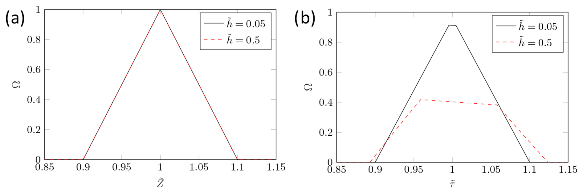
Figure 4 presents the transfer functions for $\stackrel{\mathrm{̃}}{\mathit{\tau }}=\mathrm{0}$ and $\stackrel{\mathrm{̃}}{Z}=\mathrm{0}$ of the CDMA. For $\stackrel{\mathrm{̃}}{\mathit{\tau }}=\mathrm{0}$ (Fig. 4a), the transfer function becomes that of a normal DMA. This is indicated by the typical triangular shape, where the FWHM (full width at half maximum) value also corresponds to the value for β. It can also be seen that there is no dependence on the slit geometry, because the curves for both $\stackrel{\mathrm{̃}}{h}=\mathrm{0.05}$ and $\stackrel{\mathrm{̃}}{h}=\mathrm{0.5}$ are identical.

The transfer function for $\stackrel{\mathrm{̃}}{Z}=\mathrm{0}$ (Fig. 4b) exhibits pure AAC behaviour. In contrast to traditional AAC theory (Tavakoli and Olfert, 2014), the transfer function does not have a triangular shape. This is due to the assumption of a mean centrifugal force acting on the particles throughout the whole classification gap, which has been used thus far. However, as described in the previous section, increased particle deposition occurs because the centrifugal force increases with an increasing radius. This means that, if particles with $\stackrel{\mathrm{̃}}{\mathit{\tau }}=\mathrm{1}$ are fed over the inlet, all particle trajectories should only be shifted parallel. However, as the centrifugal force increases with radius, particles entering the classifier gap at a larger radius are directly affected by a higher centrifugal force. Thus, if the particles are close to r₂, they are already located at a larger radius compared to the centre radius of the aerosol inlet when they enter the transfer zone, so they experience a higher centrifugal force. Figure 5a shows individual particle trajectories (with $\stackrel{\mathrm{̃}}{\mathit{\tau }}=\mathrm{1}$ and $\stackrel{\mathrm{̃}}{Z}=\mathrm{0}$) for particles fed between r₁ and r₂ (blue dashed line) and sampled between r₃ and r₄ (the two red dashed lines) after transfer length L.

It can be seen that the particle trajectories are widened to such an extent that particles are deposited both before and after the sampling gap – particle trajectories which do not end between the red lines at L are deposited on the walls before or after the sampling outlet. This phenomenon is, of course, due to the way in which the AAC works and therefore occurs mainly when the particle relaxation time is relevant. This is also why the ideal transfer function for an AAC is a truncated triangular function. This increases as the $\stackrel{\mathrm{̃}}{h}$ value increases, so the shape of the transfer function becomes increasingly distorted and values for Ω decline.

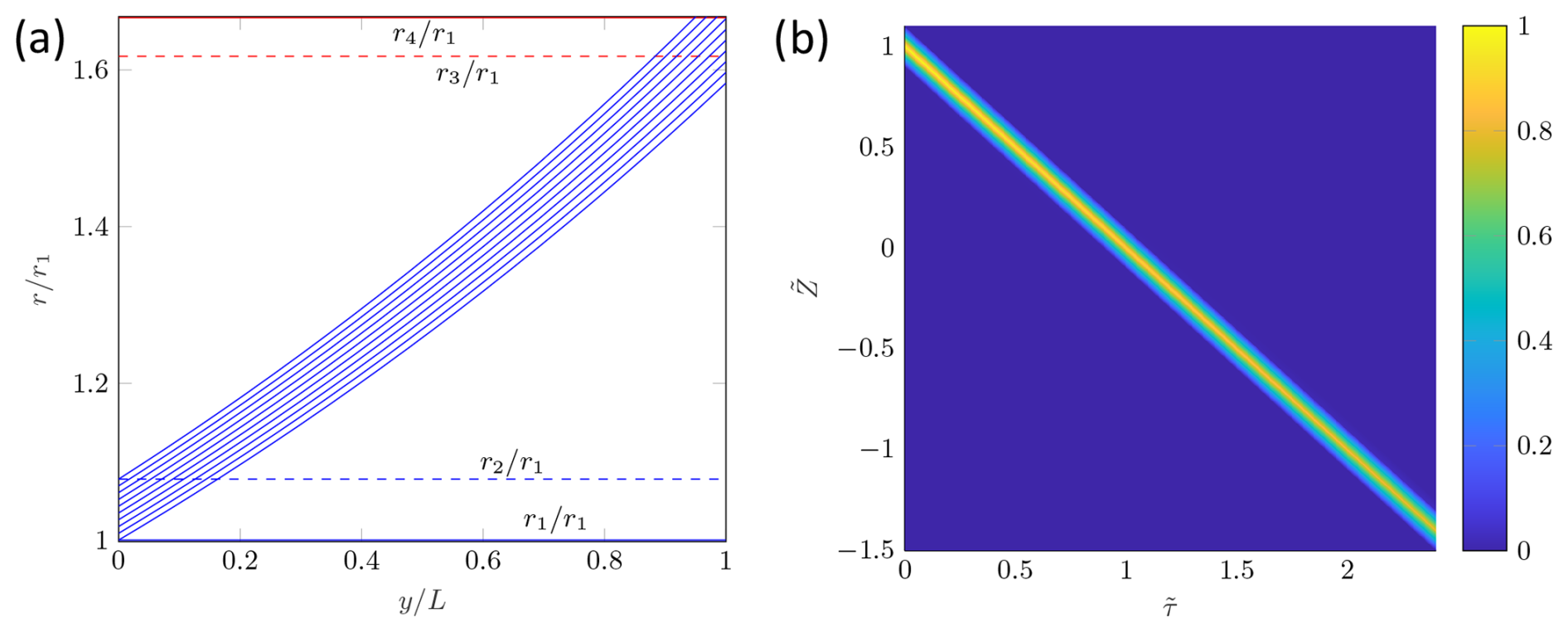
Figure 5 Exemplary particle trajectories for $\stackrel{\mathrm{̃}}{Z}=\mathrm{0}$, $\stackrel{\mathrm{̃}}{\mathit{\tau }}=\mathrm{1}$, and $\stackrel{\mathrm{̃}}{h}=\mathrm{0.5}$ (a) and 2D transfer functions β=0.1 and $\stackrel{\mathrm{̃}}{h}=\mathrm{0.05}$.

4.3 Theoretical 2D transfer function

Equation (11) can be used to calculate the transfer probability for each combination of $\stackrel{\mathrm{̃}}{\mathit{\tau }}$ and $\stackrel{\mathrm{̃}}{Z}$. If β=0.1 and $\stackrel{\mathrm{̃}}{h}=\mathrm{0.05}$, the 2D transfer function shown in Fig. 5b is obtained. Here, the influence of the widening particle trajectories increases with decreasing $\stackrel{\mathrm{̃}}{Z}$ and increasing values of $\stackrel{\mathrm{̃}}{\mathit{\tau }}$, and the height of the transfer function decreases. It should be noted that, in contrast to $\stackrel{\mathrm{̃}}{\mathit{\tau }}$, there are also negative values for $\stackrel{\mathrm{̃}}{Z}$. This is due to the presence of both positively and negatively charged particles. For $\stackrel{\mathrm{̃}}{Z}>\mathrm{0}$, the direction of the electrical force is on the particles with the centrifugal force. For $\stackrel{\mathrm{̃}}{Z}<\mathrm{0}$, it acts in the opposite direction. Using the 2D transfer function, the classification probabilities can be calculated for each operating point, providing a matrix for data inversion, which is required for back-calculation.

5 Measurement of the transfer functions for the DMA and AAC operating modes

To validate the instrument functionality, the transfer functions for $\stackrel{\mathrm{̃}}{\mathit{\tau }}=\mathrm{0}$ and $\stackrel{\mathrm{̃}}{Z}=\mathrm{0}$ (DMA mode, i.e. ω=0; AAC mode, i.e. U=0) should first be determined experimentally. To measure a DMA–AAC transfer function, a tandem setup consisting of two instruments was used, where the first instrument continuously provides a mono-mobile aerosol while the second instrument scans the whole measuring range step by step.

In this case, a classifier (TSI 3080) with a DMA (TSI 3081) and a Kr-85 neutralizer (TSI 3077a) was used as the first instrument in the tandem setup, providing the mono-mobile aerosol. The voltage and desired volume flows are set there. To investigate the different operation parameters, Q_a was set to 0.3 or 1.5 lpm and Q_sh was varied between 1.5 lpm and about 20 lpm, resulting in different values for β. The second device was the CDMA, to which the same volume flows are applied via another classifier (TSI 3080). The used classifiers include a negative voltage power supply, so that both devices sample positively charged particles. To measure the transfer function, the measuring range of the CDMA is scanned step by step. That is, the voltage or speed is increased discretely and the resulting concentration n₂ is measured. As the concentration after the first unit (n₁) is also important for the calculation, the second unit can be bypassed using two valves. For the aerosol production, two tube furnaces and an agglomeration tube are used. Figure 6 shows a scheme of this complete setup.

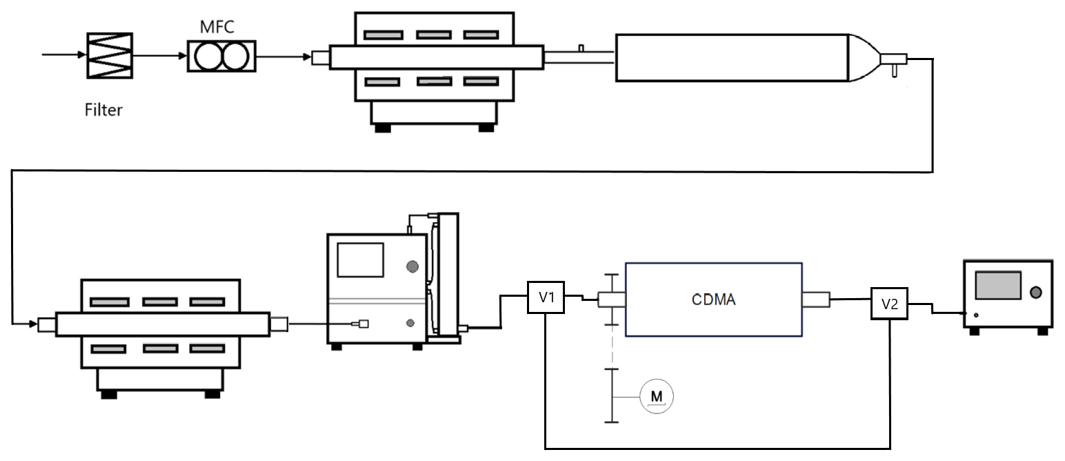
Figure 6 Schematic of the entire experimental setup: test aerosol production with two tube furnaces (Nabertherm) and an agglomeration tube, together with the consecutive setup consisting of a classifier (TSI 3080) with a DMA (TSI 3081), CDMA (TSI 3775), and CPC (TSI 3775) for the measurement of a transfer function.

5.1 Production of a test aerosol

To obtain meaningful measurements, it is also important to produce a stable and constant test aerosol. This is achieved by heating silver to 1150 °C in a hot-wall reactor. During this process, some of the silver evaporates into the gas phase. When the temperature is lowered at the outlet of the hot-wall reactor, silver vapor nucleates to form nanoparticles. Larger agglomerates are formed in the agglomeration tube.

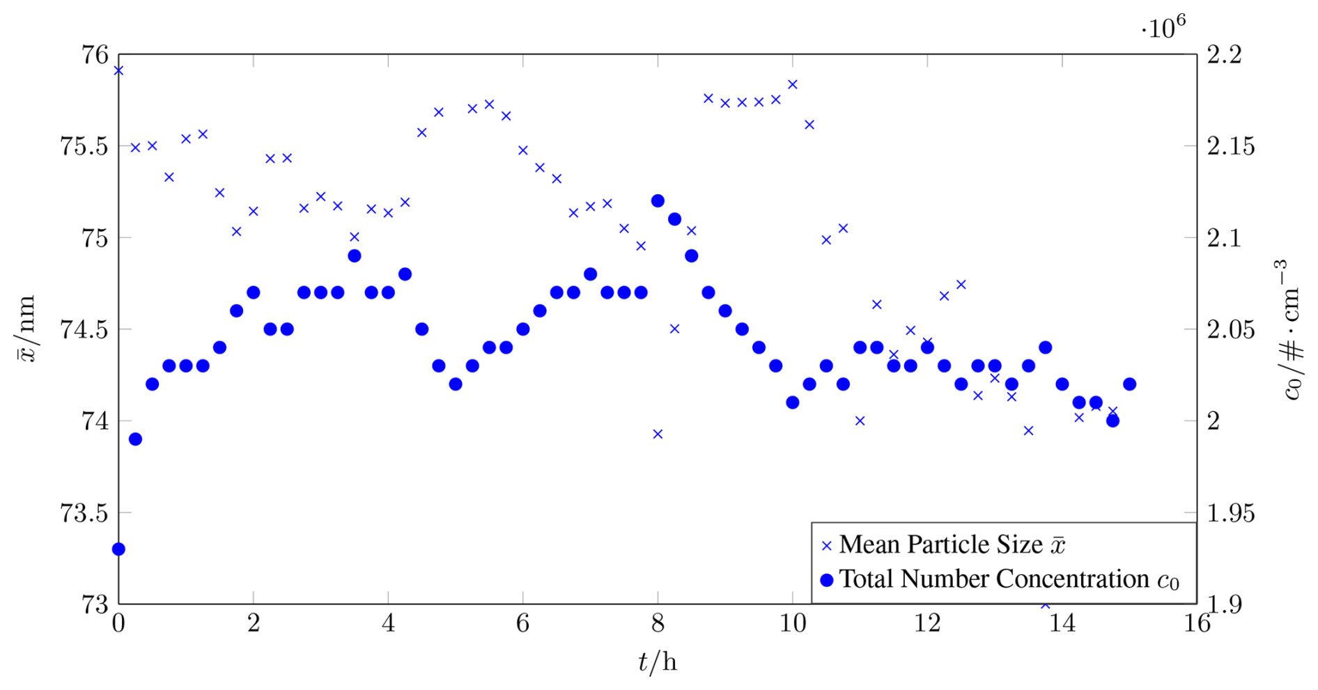
These agglomerates can be heated to approximately 700 °C in a second hot-wall reactor in order to thermally round them into spherical particles. Figure 7 shows the mean particle diameter of the test aerosol after agglomeration. It can be seen that the mean particle size and total number concentration remain very stable over a long period of time, allowing us to measure transfer functions, which typically takes about 30 min. Figure 8a shows the roundness of the particles and thus underscores their suitability for the first CDMA evaluation.

Figure 7 Mean particle diameter and total concentration measured by the SMPS over time.

5.2 Calculating a transfer function from measurement data assuming a Gaussian shape

If the tubing length from the first valve (V1) to the second instrument plus the tubing length from the second instrument to the second valve (V2) is equal to the length of the tubing, which is the bypass of the second instrument, the tubing loss term is eliminated (Li et al., 2006). The efficiency of the condensation particle counter (CPC) is also eliminated if exactly the same CPC is used to measure n₁ and n₂ (see Fig. 6 and Sect. 5).

Since the first instrument is a DMA, the determination of the transfer function for the DMA mode (i.e. ω=0) is done in the following. For the quotient $n_{\mathrm{2}}/n_{\mathrm{1}}$, the following formula applies (Li et al., 2006)⁴:

$$\begin{array}{}\text{(16)}& n_{\mathrm{2}}/n_{\mathrm{1}}={\displaystyle \frac{\underset{-\mathrm{\infty }}{\overset{+\mathrm{\infty }}{\int }}{\mathrm{\Omega }}_{\mathrm{1}}\left(\stackrel{\mathrm{̃}}{Z}\right)\cdot {\mathrm{\Omega }}_{\mathrm{2}}\left(\stackrel{\mathrm{̃}}{Z}\right)\mathrm{d}\stackrel{\mathrm{̃}}{Z}}{\underset{-\mathrm{\infty }}{\overset{+\mathrm{\infty }}{\int }}{\mathrm{\Omega }}_{\mathrm{1}}\left(\stackrel{\mathrm{̃}}{Z}\right)\mathrm{d}\stackrel{\mathrm{̃}}{Z}}}.\end{array}$$

Here, Ω₁ and Ω₂ represent the transfer functions of the first and second measurement devices.

Deviating from the ideal type assumption of the previously discussed triangular transfer function, a Gaussian function is now assumed for the shape of the transfer function. This approach is sensible for considering the effects of diffusion or the lack of a plugflow profile in the inlet gap. Moreover, the convolution of two Gaussian functions is also a Gaussian function, which fits very well with the measurement data (Fig. 8b).

A Gaussian transfer function can be described by

$$\begin{array}{}\text{(17)}& \begin{array}{rl}& {\mathrm{\Omega }}_{\mathrm{1}}=a\cdot \exp \left\{-{\displaystyle \frac{(\stackrel{\mathrm{̃}}{Z}-{\stackrel{\mathrm{̃}}{\mathit{\mu }}}_{\mathrm{1}}{)}^{\mathrm{2}}}{c^{\mathrm{2}}}}\right\},\\ & {\mathrm{\Omega }}_{\mathrm{2}}=d\cdot \exp \left\{-{\displaystyle \frac{(\stackrel{\mathrm{̃}}{Z}-{\stackrel{\mathrm{̃}}{\mathit{\mu }}}_{\mathrm{2}}{)}^{\mathrm{2}}}{e^{\mathrm{2}}}}\right\},\end{array}\end{array}$$

where a and d are transfer function height fit parameters, ${\stackrel{\mathrm{̃}}{\mathit{\mu }}}_{\mathrm{2}}$ is a transfer function position fit parameter, and e is a transfer function width fit parameter. In the normalized case, the position fit parameters ${\stackrel{\mathrm{̃}}{\mathit{\mu }}}_{\mathrm{1}}$ and ${\stackrel{\mathrm{̃}}{\mathit{\mu }}}_{\mathrm{2}}$ should be 1, but for real measurements there are some minor errors or inaccuracies that can be determined by these parameters. Since the position of the function on the abscissa is inconsequential when integrating from −∞ to +∞, the abscissa can be displaced arbitrarily. If the abscissa is now displaced so that the centre of the first transfer function is zero, the following equation is obtained:

$$\begin{array}{}\text{(18)}& \begin{array}{rl}& n_{\mathrm{2}}/n_{\mathrm{1}}=\\ & {\displaystyle \frac{\underset{-\mathrm{\infty }}{\overset{+\mathrm{\infty }}{\int }}a\cdot \exp \left\{-\frac{{\stackrel{\mathrm{̃}}{Z}}^{\mathrm{2}}}{c^{\mathrm{2}}}\right\}\cdot d\cdot \exp \left\{-\frac{(\stackrel{\mathrm{̃}}{Z}-{\stackrel{\mathrm{̃}}{\mathit{\mu }}}_{\mathrm{2}}+{\stackrel{\mathrm{̃}}{\mathit{\mu }}}_{\mathrm{1}}{)}^{\mathrm{2}}}{e^{\mathrm{2}}}\right\}\mathrm{d}\stackrel{\mathrm{̃}}{Z}}{\underset{-\mathrm{\infty }}{\overset{+\mathrm{\infty }}{\int }}a\cdot \exp \left\{-\frac{{\stackrel{\mathrm{̃}}{Z}}^{\mathrm{2}}}{c^{\mathrm{2}}}\right\}\mathrm{d}\stackrel{\mathrm{̃}}{Z}}}.\end{array}\end{array}$$

Solving these integrals,

$$\begin{array}{}\text{(19)}& \begin{array}{rl}& \underset{-\mathrm{\infty }}{\overset{+\mathrm{\infty }}{\int }}a\cdot \exp \left\{-{\displaystyle \frac{{\stackrel{\mathrm{̃}}{Z}}^{\mathrm{2}}}{c^{\mathrm{2}}}}\right\}\cdot d\cdot \exp \left\{-{\displaystyle \frac{(\stackrel{\mathrm{̃}}{Z}-{\stackrel{\mathrm{̃}}{\mathit{\mu }}}_{\mathrm{2}}+{\stackrel{\mathrm{̃}}{\mathit{\mu }}}_{\mathrm{1}}{)}^{\mathrm{2}}}{e^{\mathrm{2}}}}\right\}\mathrm{d}\stackrel{\mathrm{̃}}{Z}\\ & =\sqrt{{\displaystyle \frac{\mathit{\pi }}{c^{\mathrm{2}}+e^{\mathrm{2}}}}}\cdot a\cdot d\cdot \left|c\right|\cdot \left|e\right|\cdot \exp \left\{-{\displaystyle \frac{({\stackrel{\mathrm{̃}}{\mathit{\mu }}}_{\mathrm{2}}-{\stackrel{\mathrm{̃}}{\mathit{\mu }}}_{\mathrm{1}}{)}^{\mathrm{2}}}{c^{\mathrm{2}}+e^{\mathrm{2}}}}\right\},\end{array}\end{array}$$

$$\begin{array}{}\text{(20)}& \underset{-\mathrm{\infty }}{\overset{+\mathrm{\infty }}{\int }}a\cdot \exp \left\{-{\displaystyle \frac{{\stackrel{\mathrm{̃}}{Z}}^{\mathrm{2}}}{c^{\mathrm{2}}}}\right\}\mathrm{d}\stackrel{\mathrm{̃}}{Z}=\sqrt{\mathit{\pi }}\cdot a\cdot \left|c\right|.\end{array}$$

If the transfer function, i.e. a and c, of the first instrument is known, with the help of

$$\begin{array}{}\text{(21)}& n_{\mathrm{2}}/n_{\mathrm{1}}=\sqrt{{\displaystyle \frac{\mathrm{1}}{c^{\mathrm{2}}+e^{\mathrm{2}}}}}\cdot d\cdot \left|e\right|\cdot \exp \left\{-{\displaystyle \frac{({\stackrel{\mathrm{̃}}{\mathit{\mu }}}_{\mathrm{2}}-{\stackrel{\mathrm{̃}}{\mathit{\mu }}}_{\mathrm{1}}{)}^{\mathrm{2}}}{c^{\mathrm{2}}+e^{\mathrm{2}}}}\right\}\end{array}$$

it is possible to fit a Gaussian function to the measurement values and calculate the remaining parameters by comparison of the coefficients. Figure 8b presents the real measured values and the corresponding approximation of a Gaussian function.

The proposed method is easy to use and does not require a complex minimum search for all measurement points. In addition, the error caused by the influence of the start parameters on a minimum value search is eliminated. From Eq. (21), one can see that the height of the transfer function of the pre-classifying DMA is eliminated and therefore has no influence on the measurement.

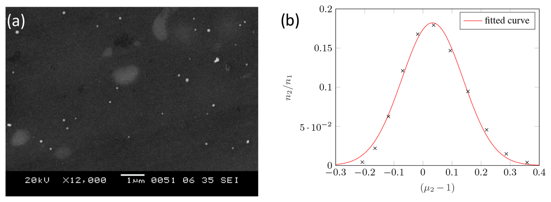
Figure 8 SEM image of silver particles (a) and a fitted Gaussian function of the ratio of the measured number concentration at the exit of the second device of the tandem setup n₂ to the number concentration at the inlet of the second device n₁, for different relative shifts of the CDMA transfer function to the fixed transfer function of the pre-classifying DMA (b).

Since the pre-classifying instrument is a DMA, the determination of the transfer function of the CDMA with U=0 V must be adopted, so that the following equations can be applied:

$$\begin{array}{}\text{(22)}& \begin{array}{rl}& {\mathrm{\Omega }}_{\mathrm{1}}=a\cdot \exp \left\{-{\displaystyle \frac{(\stackrel{\mathrm{̃}}{\mathit{\tau }}-{\stackrel{\mathrm{̃}}{\mathit{\mu }}}_{\mathrm{1}}{)}^{\mathrm{2}}}{c^{\mathrm{2}}}}\right\},\\ & {\mathrm{\Omega }}_{\mathrm{2}}=d\cdot \exp \left\{-{\displaystyle \frac{(\stackrel{\mathrm{̃}}{\mathit{\tau }}-{\stackrel{\mathrm{̃}}{\mathit{\mu }}}_{\mathrm{2}}{)}^{\mathrm{2}}}{e^{\mathrm{2}}}}\right\}.\end{array}\end{array}$$

Therefore, the transfer function for the first DMA must be determined first. This is done in Appendix C.

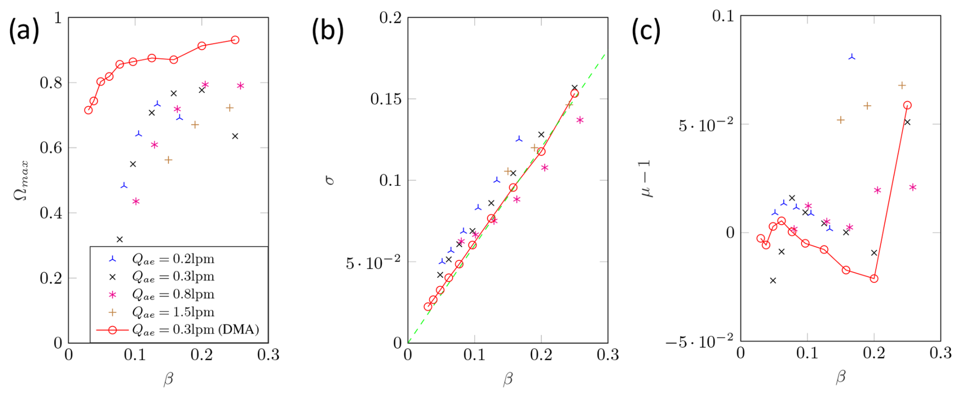
Figure 9 Measured transfer function parameters: maximum height (a), width (b), and shift (c) of the CDMA in DMA mode for d_p=100 nm.

5.3 Measurement results

In general, three different particle sizes (50, 100, and 200 nm) of spherical silver particles were analysed. Because the measured values were very similar for all the particle sizes, only the results for a particle size of 100 nm are presented here. The other sizes are shown in Appendix D. The transfer functions were determined over the full range of possible operating parameters. The aerosol flow rate was kept constant for each series of measurements, and the sheath airflow rate was varied so that the parameters could be determined for different values of β. Both the Scanning Mobility Particle Sizer (SMPS) DMA and the CDMA were operated at the same ratio of aerosol to sheath air volume flow. The points on the red lines show comparative measurements of a DMA–DMA configuration as a reference. It should also be noted that the corrections explained in Sect. 3.2 have already been applied here, so that the unwanted separation due to voltage or speed has already been eliminated.

To determine the transfer function of the pre-classifying DMA from the SMPS system, two identical DMAs were first measured in a tandem configuration. Assuming that they are equal regarding their classification properties, it is possible to determine the relevant parameters for the pre-classifying DMA for DMA measurements by

$$\begin{array}{}\text{(23)}& {\mathit{\mu }}_{\mathrm{1}}=\mathrm{1.00319};c=\mathrm{0.5868}\cdot \mathit{\beta }\end{array}$$

and for AAC measurements by

$$\begin{array}{}\text{(24)}& {\mathit{\mu }}_{\mathrm{1}}=\mathrm{1.00319};c=\mathrm{0.6468}\cdot \mathit{\beta }.\end{array}$$

5.3.1 DMA mode

Figure 9a plots the measured height of the transfer function against the aerosol-to-sheath air volume flow ratio. Comparing the measured values of the CDMA in DMA mode with the measurement values of a commercial DMA (TSI 3081), it is noticeable that the height is significantly lower. This is not surprising because the CDMA requires significantly more deflections and a longer travel distance during which particles are deposited on the walls by impaction or diffusion, respectively. The scatter of the measured values can be explained by random variations in the operation of the CDMA. For example, at low aerosol volume flows and high values of β, only very small sheath airflows occur, which are outside the normal operating range of recirculation technology and do not guarantee a reliable and uniform volume flow. A very strong drop in the height of the transfer function from β=0.1 to β=0.05 is observed. There is also a slight drop in the height of the DMA transfer function due to the increasing influence of diffusion as the transfer functions become narrower. However, this phenomenon does not explain the sharp decrease in the CDMA curves. In particular, for other particle sizes, exactly the same drop can be observed. This leads to the conclusion that there is no relevant particle loss due to diffusion or impaction, as a similar curve can be observed for all the volume flows. This indicates that further particle losses are present, but the source could not be identified yet. To investigate this problem, a new prototype with significantly shortened inlet and outlet regions of the aerosol and sample volume flow is required.

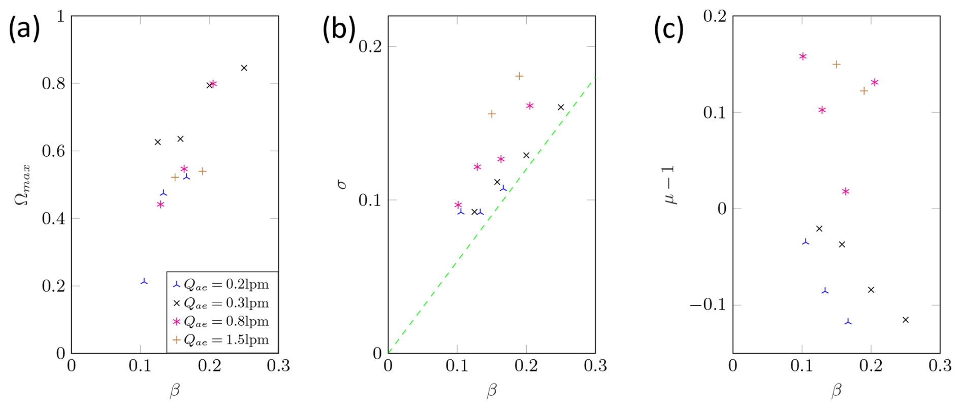
Figure 10 Measured transfer function parameters: maximum height (a), width (b), and shift (c) of the CDMA in AAC mode for d_p=100 nm.

Figure 9b shows the standard deviation of the transfer function, which corresponds to the width of the transfer function. The green dashed line represents the ideal relationship between standard deviation and β. This can also be observed in the measured values, as they too exhibit a linear dependence on β. When the measured values are compared with the DMA reference values, it is noticeable that the width of the transfer function is generally slightly larger. This can be explained by the narrower gap of the CDMA at approximately the same length (the applied voltage is therefore significantly lower and there is a lower Peclet number in the CDMA, and hence diffusion plays a greater role) and also by the assembly and tolerances of the prototype (especially in combination with the short travelling distances of the particles in the radial direction).

Figure 9c shows the shift of the transfer function on the x axis. It can be seen that there is no significant difference with the DMA comparison values. Larger deviations can be observed only for large β values. This was again due to the control range of the sheath airflow.

5.3.2 AAC mode

It should be noted that the AAC measurements have already been corrected for charge distribution. This was performed by measuring the particle size distribution available directly at the outlet of the sintering furnace. As the charge distribution is assumed to be known (Wiedensohler, 1988), it is possible to deduce the proportion of multiply charged particles that pass through the pre-classification. This fraction can then be subtracted from n₁ to obtain the actual number concentration of singly charged particles at the CDMA inlet.

Figure 10a shows the height of the transfer function for the AAC mode. Unlike the DMA mode, there is no plateau where the height remains constant. However, the transfer functions reach very high values. It can also be seen that the decrease is analogous to the heights shown for the DMA. At low β values, however, no measurement is possible, because at β<0.1 almost all particles are separated by the centrifugal force at the inlet and outlet of the CDMA.

Figure 10b again shows the standard deviation of the transfer function. There are still linear dependence on the β values and fluctuation around the ideal value. However, the scattering of the measured values was significantly larger compared to the DMA mode. This is due to the more difficult flow control as the flows take a longer distance to fully develop, i.e. due to the rotation the walls have to take with all the air in the rotation too. By changing for example the sheath air, CFD simulations have shown that the development of the flow profile is delayed in the axial direction. This effect becomes stronger as the sheath airflow rate increases. One potential improvement is the installation of vanes at the point at which the sheath radius changes. Moreover, higher angular velocities lead to a higher pressure difference at the inlet, and hence some flow disturbances may occur there. This can affect the classification zone and explains the larger variations in the results. In addition, the strong separation in the inlet and outlet areas results in very high correction factors, especially for small β values.

Figure 10c shows a similar picture to Fig. 10b. Again, the deviation is significantly greater than that in the DMA mode, which, as in Fig. 10b, is due to the flow field in CDMA. However, except for one outlier, in Fig. 10c there seems to be a linear dependence on the β values for each aerosol volume flow. In addition, the curves were all parallel, with the curves shifting in the positive direction as the aerosol volume flow increased. Again, this can be explained by the difficulty in the flow adaptation at higher speeds, i.e. higher flow velocities (or volume flows). The deviation might also be caused by manufacturing tolerances or imperfectly aligned system components. As the deviation for the other particle sizes is also very similar to this result, a calibration for the CDMA could be performed during further validation.

6 Conclusions

As described in the previous section, the transfer functions of the CDMA for $\stackrel{\mathrm{̃}}{\mathit{\tau }}=\mathrm{0}$ and $\stackrel{\mathrm{̃}}{Z}=\mathrm{0}$ agreed well with the theory and reference values of a DMA–DMA configuration. For β<0.2, the height of the transfer function decreased much more than for β>0.2, but the cause has not yet been clarified conclusively. In order to find the cause, a new prototype needs to be designed and built that significantly reduces the depositions in the inlet and outlet areas and minimizes the electrical fields outside the classification zone. The superposition of these effects makes it difficult to determine the cause in the current arrangement. As one operating point is sufficient for the initial investigations, further investigations will be conducted for β=0.2. For this purpose, this operating point needs to be measured again in detail, and a calibration of the CDMA possibly needs to be carried out. Furthermore, a validation for particle sizes larger than 200 nm is necessary in order to be able to fully describe the CDMA for those larger particles. The ideal 2D transfer function can be calculated using the particle trajectory method. However, an extension to the streamline model is highly recommended for validation, because diffusion in the classifier gap can be considered. Furthermore, a new robust method of measuring transfer functions was presented, which made it possible to draw conclusions about the transfer function simply by measuring the number concentrations. If these results agree with the theoretical values for different particle types, the final step is to develop an algorithm that can be used to calculate a 2D distribution with respect to d_m and d_st from the measured values.

Appendix A: Comment on the definition of the particle relaxation time

In contrast to Tavakoli and Olfert (2014), the Stokes equivalent diameter was used instead of the aerodynamic-equivalent diameter. Furthermore, the argument of the Cunningham slip correction should be mentioned here. The equations for calculating the slip correction are derived only for spherical particles. There are many studies in the literature dealing with the slip correction for non-spherical particles. For example, Cheng et al. (1988) and Dahneke (1973) proposed the introduction of a new equivalent diameter for non-spherical particles with the same slip correction. However, these methods are mostly limited to specific particle shapes and apply only to the free molecular or continuum region but not to the transition region. However, we consider the aerodynamic-equivalent diameter to be inappropriate for calculating the slip correction as done by Tavakoli and Olfert (2014), since the aerodynamic diameter depends on the particle density as well. That is, two particles with identical shapes but different densities would experience the same drag force and thus slip correction while having different aerodynamic diameters. Therefore, we suggest using the mobility-equivalent diameter instead. This is in accordance with a number of studies in the literature, such as Knutson and Whitby (1975) and Sorensen (2011). Moreover, slip correction experimental investigations have typically been performed using the Millikan apparatus, where the particles are moved in an electrical field (Buckley and Loyalka, 1989; Rader, 1990; Allen and Raabe, 1985).

Appendix B: Derivation of the 2D transfer function using particle trajectory calculation

In accordance with the specified operating parameters (i.e. voltage U and speed ω), a multitude of combinations of the equivalent particle sizes d_m and d_st or combinations of τ and Z can be derived analytically from the geometry and the volume flow conditions. The aforementioned combinations are subject to a probability of classification. A characteristic combination, for instance, exhibits the property that, if a particle is introduced at the centre of the inlet gap, it will also be collected at the centre of the classifying gap. In the case of edge transfer functions, the following relationships are observed: $\mathit{\tau }={\mathit{\tau }}^{*}$ or $\stackrel{\mathrm{̃}}{\mathit{\tau }}=\mathrm{1}$ (for $Z^{*}=\mathrm{0}$) and $Z=Z^{*}$, or $\stackrel{\mathrm{̃}}{Z}=\mathrm{1}$ (for ${\mathit{\tau }}^{*}=\mathrm{0}$). The results are presented in Sect. 4.2 of this article.

Two characteristic classification properties are the limiting particle trajectories, hereafter called the maximum and minimum particle paths. All particles that traverse the classifying section at a shorter distance than the particle on the minimum path are no longer classified. This minimum path is defined by substituting r_in=r₂ and r(L)=r₃ into Eq. (9). In contrast, the maximum particle trajectory represents the boundary from which particles traversing a greater distance are deposited at the inner electrode (r_in=r₁ and r(L)=r₄). Equation (9) may be employed to ascertain the transfer probability for each τ–Z combination. If two critical radii (r_c) are defined where $r_{\mathrm{1}}<r_{\mathrm{c}}<r_{c\mathrm{2}}<r_{\mathrm{2}}$ and a constant particle flux density at the inlet is assumed, the transfer probability can be determined by the following equations:

$$\begin{array}{}\text{(B1)}& {\mathrm{\Omega }}_{\mathrm{CDMA}}=\max \left[\min \left(f_{\mathrm{1}},f_{\mathrm{2}},\mathrm{1}\right),\mathrm{0}\right],\end{array}$$

$$\begin{array}{}\text{(B2)}& f_{\mathrm{1}}={\displaystyle \frac{r_{\mathrm{2}}^{\mathrm{2}}-r_c^{\mathrm{2}}}{r_{\mathrm{2}}^{\mathrm{2}}-r_{\mathrm{1}}^{\mathrm{2}}}}-\max \left({\displaystyle \frac{r_{\mathrm{2}}^{\mathrm{2}}-r_{c\mathrm{2}}^{\mathrm{2}}}{r_{\mathrm{2}}^{\mathrm{2}}-r_{\mathrm{1}}^{\mathrm{2}}}},\mathrm{0}\right),\end{array}$$

$$\begin{array}{}\text{(B3)}& f_{\mathrm{2}}={\displaystyle \frac{r_{\mathrm{c}\mathrm{2}}^{\mathrm{2}}-r_{\mathrm{1}}^{\mathrm{2}}}{r_{\mathrm{2}}^{\mathrm{2}}-r_{\mathrm{1}}^{\mathrm{2}}}}-\max \left({\displaystyle \frac{r_{\mathrm{c}}^{\mathrm{2}}-r_{\mathrm{1}}^{\mathrm{2}}}{r_{\mathrm{2}}^{\mathrm{2}}-r_{\mathrm{1}}^{\mathrm{2}}}},\mathrm{0}\right).\end{array}$$

In other words, if we assume that the minimum particle path is limiting (as is the case for f₁ with the DMA transfer function; Wang and Flagan, 1990), a lower critical radius can be defined so that all particles entering at r<r_c are no longer classified but are separated behind the classifying gap or discharged with the sheath air.

Therefore, r_c is defined by

$$\begin{array}{}\text{(B4)}& r_{\mathrm{3}}=\sqrt{r_{\mathrm{c}}^{\mathrm{2}}\cdot \exp \left\{\stackrel{\mathrm{̃}}{\mathit{\tau }}\cdot {\displaystyle \frac{\mathrm{2}\stackrel{\mathrm{̃}}{h}}{\mathrm{1}+\mathit{\beta }}}\right\}+{\stackrel{\mathrm{‾}}{r}}^{\mathrm{2}}\cdot {\displaystyle \frac{\stackrel{\mathrm{̃}}{Z}}{\stackrel{\mathrm{̃}}{\mathit{\tau }}}}\cdot \left[\exp \left\{\stackrel{\mathrm{̃}}{\mathit{\tau }}\cdot {\displaystyle \frac{\mathrm{2}\stackrel{\mathrm{̃}}{h}}{\mathrm{1}+\mathit{\beta }}}\right\}-\mathrm{1}\right]}.\end{array}$$

As a consequence of the speed-controlled operating mode, it is possible that not all particles entering at r₂ will be classified. Because of the elevated feed radius, a higher drift velocity is observed at the outlet of the transfer section, thereby enabling the separation of particles at the outer electrode or excess air (for further details, please refer to Sect. 4.2). In order to accommodate this phenomenon, a second critical radius, designated as r_c2, is introduced, situated between r_c and r₂; the calculation is performed in accordance with the following formula:

$$\begin{array}{}\text{(B5)}& r_{\mathrm{4}}=\sqrt{r_{\mathrm{c}\mathrm{2}}^{\mathrm{2}}\cdot \exp \left\{\stackrel{\mathrm{̃}}{\mathit{\tau }}\cdot {\displaystyle \frac{\mathrm{2}\stackrel{\mathrm{̃}}{h}}{\mathrm{1}+\mathit{\beta }}}\right\}+{\stackrel{\mathrm{‾}}{r}}^{\mathrm{2}}\cdot {\displaystyle \frac{\stackrel{\mathrm{̃}}{Z}}{\stackrel{\mathrm{̃}}{\mathit{\tau }}}}\cdot \left[\exp \left\{\stackrel{\mathrm{̃}}{\mathit{\tau }}\cdot {\displaystyle \frac{\mathrm{2}\stackrel{\mathrm{̃}}{h}}{\mathrm{1}+\mathit{\beta }}}\right\}-\mathrm{1}\right]}.\end{array}$$

Once the flow ratio β has been established, it can be subtracted from the initial value in order to prevent the value r_c2 from exceeding r₂. The minimum value for this term is set to 0.

In light of the continuously increasing probability of transfer in the direction of r₁, a new parameter (f₂) is introduced. It is important to note that the maximum particle path represents a limiting quantity too. The same procedure is applied as for f₁, but now r_c2 is used as the critical radius for the first term, while r_c is used for the second term. This implies that all particles entering the transfer section with a radius greater than r_c2 are separated at the outer electrode before the classification gap. As a consequence of the reduction in radius, particles entering the transfer section at r_in>r₁ are again subjected to separation. A second critical radius is defined at which the particles are classified. The area ratio can once more be subtracted from the first term. Since the case r_c<r₁ cannot occur, a value of zero is also defined here as the minimum.

.

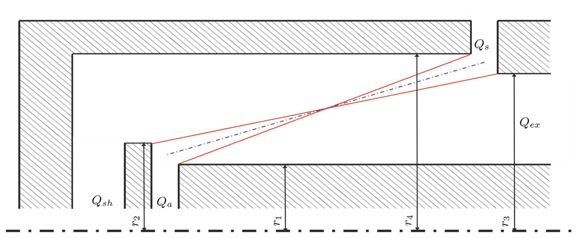
Figure B1 Characteristic particle paths: minimal and maximal particle paths (solid red lines) and the centred particle path (dash-dotted blue line) for combinations of τ and Z

The probability of a τ–Z combination being classified is now the smaller of f₁ or f₂. This is due to the fact that both the maximum and minimum particle paths were taken into account. Furthermore, it should be noted that the transfer function can assume a maximum value of 1. It is also necessary to ensure that the transfer function does not become smaller than 0. This implies that the minima of f₁, f₂, and 1 must not become smaller than 0 (Eq. 11).

Upon substituting Eqs. (B4) and (B5) into Eqs. (B2) and (B3), the following result is obtained:

$$\begin{array}{}\text{(B6)}& \begin{array}{rl}& f_{\mathrm{1}}={\displaystyle \frac{r_{\mathrm{2}}^{\mathrm{2}}-\left(r_{\mathrm{3}}^{\mathrm{2}}+{\stackrel{\mathrm{‾}}{r}}^{\mathrm{2}}\cdot \frac{\stackrel{\mathrm{̃}}{Z}}{\stackrel{\mathrm{̃}}{\mathit{\tau }}}\right)\cdot \exp \left\{-\stackrel{\mathrm{̃}}{\mathit{\tau }}\cdot \frac{\mathrm{2}\stackrel{\mathrm{̃}}{h}}{\mathrm{1}+\mathit{\beta }}\right\}{\stackrel{\mathrm{‾}}{r}}^{\mathrm{2}}\cdot \frac{\stackrel{\mathrm{̃}}{Z}}{\stackrel{\mathrm{̃}}{\mathit{\tau }}}}{r_{\mathrm{2}}^{\mathrm{2}}-r_{\mathrm{1}}^{\mathrm{2}}}}\\ & -\max \left({\displaystyle \frac{r_{\mathrm{2}}^{\mathrm{2}}-\left(r_{\mathrm{4}}^{\mathrm{2}}+{\stackrel{\mathrm{‾}}{r}}^{\mathrm{2}}\cdot \frac{\stackrel{\mathrm{̃}}{Z}}{\stackrel{\mathrm{̃}}{\mathit{\tau }}}\right)\cdot \exp \left\{-\stackrel{\mathrm{̃}}{\mathit{\tau }}\cdot \frac{\mathrm{2}\stackrel{\mathrm{̃}}{h}}{\mathrm{1}+\mathit{\beta }}\right\}+{\stackrel{\mathrm{‾}}{r}}^{\mathrm{2}}\cdot \frac{\stackrel{\mathrm{̃}}{Z}}{\stackrel{\mathrm{̃}}{\mathit{\tau }}}}{r_{\mathrm{2}}^{\mathrm{2}}-r_{\mathrm{1}}^{\mathrm{2}}}},\mathrm{0}\right),\end{array}\end{array}$$

$$\begin{array}{}\text{(B7)}& \begin{array}{rl}& f_{\mathrm{2}}={\displaystyle \frac{\left(r_{\mathrm{4}}^{\mathrm{2}}+{\stackrel{\mathrm{‾}}{r}}^{\mathrm{2}}\cdot \frac{\stackrel{\mathrm{̃}}{Z}}{\stackrel{\mathrm{̃}}{\mathit{\tau }}}\right)\cdot \exp \left\{-\stackrel{\mathrm{̃}}{\mathit{\tau }}\cdot \frac{\mathrm{2}\stackrel{\mathrm{̃}}{h}}{\mathrm{1}+\mathit{\beta }}\right\}-{\stackrel{\mathrm{‾}}{r}}^{\mathrm{2}}\cdot \frac{\stackrel{\mathrm{̃}}{Z}}{\stackrel{\mathrm{̃}}{\mathit{\tau }}}-r_{\mathrm{1}}^{\mathrm{2}}}{r_{\mathrm{2}}^{\mathrm{2}}-r_{\mathrm{1}}^{\mathrm{2}}}}\\ & -\max \left({\displaystyle \frac{(r_{\mathrm{3}}^{\mathrm{2}}+{\stackrel{\mathrm{‾}}{r}}^{\mathrm{2}}\cdot \frac{\stackrel{\mathrm{̃}}{Z}}{\stackrel{\mathrm{̃}}{\mathit{\tau }}})\cdot \exp \left\{-\stackrel{\mathrm{̃}}{\mathit{\tau }}\cdot \frac{\mathrm{2}\stackrel{\mathrm{̃}}{h}}{\mathrm{1}+\mathit{\beta }}\right\}-{\stackrel{\mathrm{‾}}{r}}^{\mathrm{2}}\cdot \frac{\stackrel{\mathrm{̃}}{Z}}{\stackrel{\mathrm{̃}}{\mathit{\tau }}}-r_{\mathrm{1}}^{\mathrm{2}}}{r_{\mathrm{2}}^{\mathrm{2}}-r_{\mathrm{1}}^{\mathrm{2}}}},\mathrm{0}\right).\end{array}\end{array}$$

Assuming a constant flux density at the inlet, the radii can be set in relation to each other. This yields the following relationships:

$$\begin{array}{}\text{(B8)}& \begin{array}{rl}& u={\displaystyle \frac{Q_{\mathrm{sh}}+Q_{\mathrm{a}}}{\mathit{\pi }(r_{\mathrm{4}}^{\mathrm{2}}-r_{\mathrm{1}}^{\mathrm{2}})}}={\displaystyle \frac{Q_{\mathrm{sh}}}{\mathit{\pi }(r_{\mathrm{4}}^{\mathrm{2}}-r_{\mathrm{2}}^{\mathrm{2}})}}={\displaystyle \frac{Q_{\mathrm{a}}}{\mathit{\pi }(r_{\mathrm{2}}^{\mathrm{2}}-r_{\mathrm{1}}^{\mathrm{2}})}}\\ & ={\displaystyle \frac{Q_{\mathrm{ex}}}{\mathit{\pi }(r_{\mathrm{3}}^{\mathrm{2}}-r_{\mathrm{1}}^{\mathrm{2}})}}={\displaystyle \frac{Q_{\mathrm{s}}}{\mathit{\pi }(r_{\mathrm{4}}^{\mathrm{2}}-r_{\mathrm{3}}^{\mathrm{2}})}}.\end{array}\end{array}$$

Using these relations for the typical operation conditions (Q_a=Q_s and subsequently Q_sh=Q_ex) and $\mathit{\beta }=Q_{\mathrm{a}}/Q_{\mathrm{sh}}$ can lead to

$$\begin{array}{}\text{(B9)}& \begin{array}{rl}& {\left({\displaystyle \frac{r_{\mathrm{2}}}{r_{\mathrm{4}}}}\right)}^{\mathrm{2}}={\displaystyle \frac{\mathit{\beta }+{\mathit{\kappa }}^{\mathrm{2}}}{\mathrm{1}+\mathit{\beta }}},\\ & {\left({\displaystyle \frac{r_{\mathrm{3}}}{r_{\mathrm{4}}}}\right)}^{\mathrm{2}}={\displaystyle \frac{\mathrm{1}/\mathit{\beta }+{\mathit{\kappa }}^{\mathrm{2}}}{\mathrm{1}/\mathit{\beta }+\mathrm{1}}},\\ & {\left({\displaystyle \frac{\stackrel{\mathrm{‾}}{r}}{r_{\mathrm{4}}}}\right)}^{\mathrm{2}}={\displaystyle \frac{(\mathit{\kappa }+\mathrm{1}{)}^{\mathrm{2}}}{\mathrm{4}}},\end{array}\end{array}$$

with

$$\begin{array}{}\text{(B10)}& \mathit{\kappa }={\displaystyle \frac{r_{\mathrm{1}}}{r_{\mathrm{4}}}}={\displaystyle \frac{\mathrm{1}-\stackrel{\mathrm{̃}}{h}/\mathrm{2}}{\mathrm{1}+\stackrel{\mathrm{̃}}{h}/\mathrm{2}}}.\end{array}$$

In order to insert the ratios from Eqs. (9) and (10), it is necessary to expand the denominator and numerator with $r_{\mathrm{4}}^{\mathrm{2}}$ in Eqs. (7) and (8). From this follows, for f₁ and f₂,

$$\begin{array}{}\text{(B11)}& \begin{array}{rl}& f_{\mathrm{1}}={\displaystyle \frac{\frac{\mathit{\beta }+{\mathit{\kappa }}^{\mathrm{2}}}{\mathrm{1}+\mathit{\beta }}-\left(\frac{\mathrm{1}/\mathit{\beta }+{\mathit{\kappa }}^{\mathrm{2}}}{\mathrm{1}/\mathit{\beta }+\mathrm{1}}+\frac{(\mathit{\kappa }+\mathrm{1}{)}^{\mathrm{2}}}{\mathrm{4}}\cdot \frac{\stackrel{\mathrm{̃}}{Z}}{\stackrel{\mathrm{̃}}{\mathit{\tau }}}\right)\cdot \exp \left\{-\stackrel{\mathrm{̃}}{\mathit{\tau }}\cdot \frac{\mathrm{2}\stackrel{\mathrm{̃}}{h}}{\mathrm{1}+\mathit{\beta }}\right\}+\frac{(\mathit{\kappa }+\mathrm{1}{)}^{\mathrm{2}}}{\mathrm{4}}\cdot \frac{\stackrel{\mathrm{̃}}{Z}}{\stackrel{\mathrm{̃}}{\mathit{\tau }}}}{\frac{\mathit{\beta }+{\mathit{\kappa }}^{\mathrm{2}}}{\mathrm{1}+\mathit{\beta }}-{\mathit{\kappa }}^{\mathrm{2}}}}-\\ & \max \left({\displaystyle \frac{\frac{\mathit{\beta }+{\mathit{\kappa }}^{\mathrm{2}}}{\mathit{\beta }+\mathrm{1}}-\left(\mathrm{1}+\frac{(\mathit{\kappa }+\mathrm{1}{)}^{\mathrm{2}}}{\mathrm{4}}\cdot \frac{\stackrel{\mathrm{̃}}{Z}}{\stackrel{\mathrm{̃}}{\mathit{\tau }}}\right)\cdot \exp \left\{-\stackrel{\mathrm{̃}}{\mathit{\tau }}\cdot \frac{\mathrm{2}\stackrel{\mathrm{̃}}{h}}{\mathrm{1}+\mathit{\beta }}\right\}+\frac{(\mathit{\kappa }+\mathrm{1})}{\mathrm{4}}\cdot \frac{\stackrel{\mathrm{̃}}{Z}}{\stackrel{\mathrm{̃}}{\mathit{\tau }}}}{\frac{\mathit{\beta }+{\mathit{\kappa }}^{\mathrm{2}}}{\mathrm{1}+\mathit{\beta }}-{\mathit{\kappa }}^{\mathrm{2}}}},\mathrm{0}\right),\end{array}\end{array}$$

$$\begin{array}{}\text{(B12)}& \begin{array}{rl}& f_{\mathrm{2}}={\displaystyle \frac{\left(\mathrm{1}+\frac{(\mathit{\kappa }+\mathrm{1}{)}^{\mathrm{2}}}{\mathrm{4}}\cdot \frac{\stackrel{\mathrm{̃}}{Z}}{\stackrel{\mathrm{̃}}{\mathit{\tau }}}\right)\cdot \exp \left\{-\stackrel{\mathrm{̃}}{\mathit{\tau }}\cdot \frac{\mathrm{2}\stackrel{\mathrm{̃}}{h}}{\mathrm{1}+\mathit{\beta }}\right\}-\frac{(\mathit{\kappa }+\mathrm{1}{)}^{\mathrm{2}}}{\mathrm{4}}\cdot \frac{\stackrel{\mathrm{̃}}{Z}}{\stackrel{\mathrm{̃}}{\mathit{\tau }}}-{\mathit{\kappa }}^{\mathrm{2}}}{\frac{\mathit{\beta }+{\mathit{\kappa }}^{\mathrm{2}}}{\mathrm{1}+\mathit{\beta }}-{\mathit{\kappa }}^{\mathrm{2}}}}-\\ & \max \left({\displaystyle \frac{\left(\frac{\mathrm{1}/\mathit{\beta }+{\mathit{\kappa }}^{\mathrm{2}}}{\mathrm{1}/\mathit{\beta }+\mathrm{1}}+\frac{(\mathit{\kappa }+\mathrm{1}{)}^{\mathrm{2}}}{\mathrm{4}}\cdot \frac{\stackrel{\mathrm{̃}}{Z}}{\stackrel{\mathrm{̃}}{\mathit{\tau }}}\right)\cdot \exp \left\{-\stackrel{\mathrm{̃}}{\mathit{\tau }}\cdot \frac{\mathrm{2}\stackrel{\mathrm{̃}}{h}}{\mathrm{1}+\mathit{\beta }}\right\}-\frac{(\mathit{\kappa }+\mathrm{1}{)}^{\mathrm{2}}}{\mathrm{4}}\cdot {\mathit{\kappa }}^{\mathrm{2}}}{\frac{\mathit{\beta }+{\mathit{\kappa }}^{\mathrm{2}}}{\mathrm{1}+\mathit{\beta }}-{\mathit{\kappa }}^{\mathrm{2}}}},\mathrm{0}\right).\end{array}\end{array}$$

Appendix C: Calculation of the transfer functions of the pre-classifying DMA

To determine the transfer function of the pre-classifying DMA, two identical DMAs are measured first. It is assumed that the transfer functions are identical, which means that

$$\begin{array}{}\text{(C1)}& d=a\text{and}e=c.\end{array}$$

Also assuming that the shift $\stackrel{\mathrm{̃}}{\mathit{\mu }}$ of the DMA is the same as ${\stackrel{\mathrm{̃}}{\mathit{\mu }}}_{\mathrm{1}}$ and ${\stackrel{\mathrm{̃}}{\mathit{\mu }}}_{\mathrm{2}}$, the shift of the pre-classifying DMA can be calculated as $\stackrel{\mathrm{̃}}{\mathit{\mu }}=\left({\stackrel{\mathrm{̃}}{\mathit{\mu }}}_{\mathrm{2}}-{\stackrel{\mathrm{̃}}{\mathit{\mu }}}_{\mathrm{1}}\right)/\mathrm{2}$. In the DMA mode (i.e. ω=0), Eq. (21) can be simplified:

$$\begin{array}{}\text{(C2)}& n_{\mathrm{2}}/n_{\mathrm{1}}=\sqrt{{\displaystyle \frac{\mathrm{1}}{\mathrm{2}}}}\cdot d\cdot \exp \left\{-{\displaystyle \frac{({\stackrel{\mathrm{̃}}{\mathit{\mu }}}_{\mathrm{2}}-{\stackrel{\mathrm{̃}}{\mathit{\mu }}}_{\mathrm{1}}{)}^{\mathrm{2}}}{\mathrm{2}\cdot e^{\mathrm{2}}}}\right\}.\end{array}$$

The parameters can now be extracted by fitting a Gaussian function to the measurement data and comparing the coefficients of the fitted curve and Eq. (C2).

As already explained in Sect. 5.2, a validation of the AAC mode (i.e. ω=0) is only possible if the transfer function of the DMA can be expressed as a function of the particle relaxation time. For the measurement results $n_{\mathrm{2}}/n_{\mathrm{1}}$, the mobility must be converted into the particle relaxation time, assuming a particle shape. A renewed application of a Gaussian function enables the parameters for $\mathrm{\Omega }\left(\stackrel{\mathrm{̃}}{\mathit{\tau }}\right)$ to be determined in the same way as for the DMA mode.

An alternative approach is to plot $\mathrm{\Omega }\left(\stackrel{\mathrm{̃}}{Z}\right)$, convert the mobilities into particle relaxation times, and approximate a Gaussian function using the values in the $\mathrm{\Omega }\left(\stackrel{\mathrm{̃}}{\mathit{\tau }}\right)$ diagram. The resulting approximation is shown in Fig. C1. As illustrated in the figure, there are inconsistencies between the fitting function and the generated values, particularly in the marginal areas, since the measured distribution appears to be slightly skew. Nevertheless, the shape is relatively similar, allowing for an approximation of the curve. With the assistance of the parameters from Sect. 5.3, the width of the curve is determined to be ${\mathit{\sigma }}_{U=\mathrm{0}}=\mathrm{0.06468}$ (${\mathit{\sigma }}_{\mathit{\omega }=\mathrm{0}}=\mathrm{0.05868}$). However, for an exact calculation, the aforementioned method should be employed.

These approaches for the determination of $\mathrm{\Omega }\left(\stackrel{\mathrm{̃}}{\mathit{\tau }}\right))$ are only valid for spherical particles.

Figure C1 Fit of a Gaussian function to the Ω–$\stackrel{\mathrm{̃}}{\mathit{\tau }}$ domain, based on the mobility measurements.

Appendix D: Measurement values for the determination of the pre-classifying DMA parameters

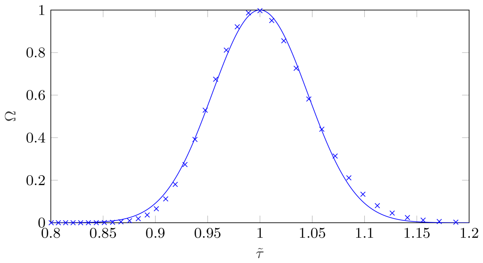
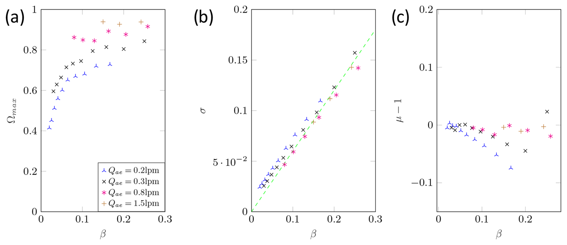
Figure D1 Measured transfer function parameters: maximum height (a), width (b), and shift (c) of the pre-classifying DMA for d_p=50 nm.

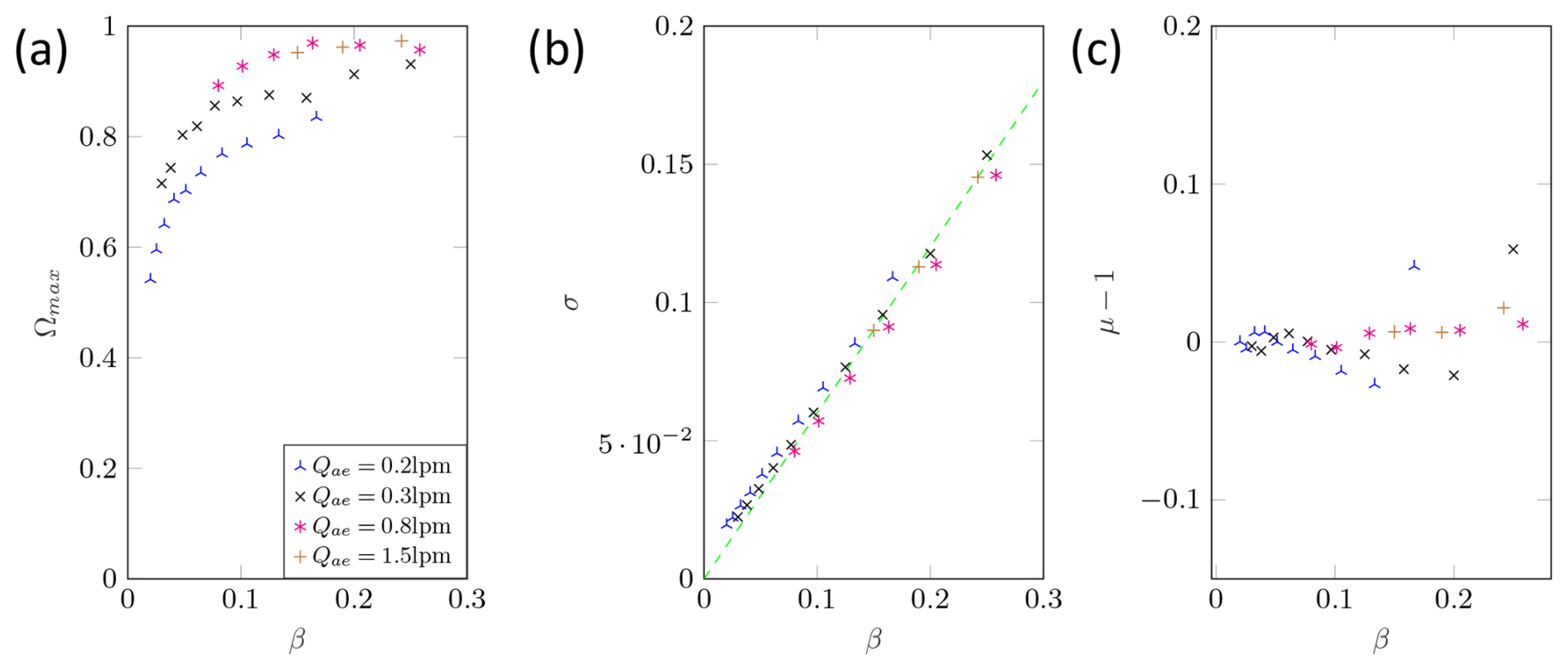
Figure D2 Measured transfer function parameters: maximum height (a), width (b), and shift (c) of the pre-classifying DMA for d_p=100 nm.

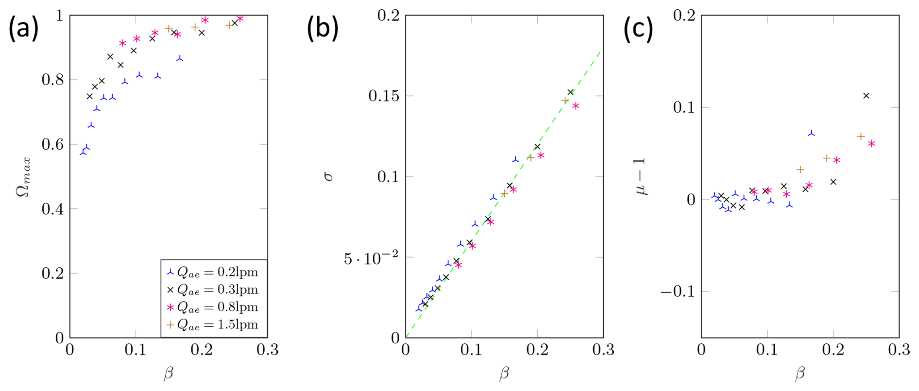
Figure D3 Measured transfer function parameters: maximum height (a), width (b), and shift (c) of the pre-classifying DMA for d_p=200 nm.

Appendix E: Measurement values for 50 and 200 nm

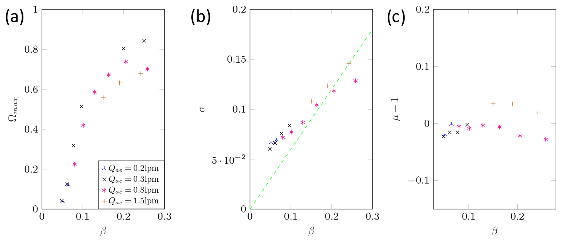
Figure E1 Measured transfer function parameters: maximum height (a), width (b), and shift (c) of the CDMA in DMA mode for d_p=50 nm.

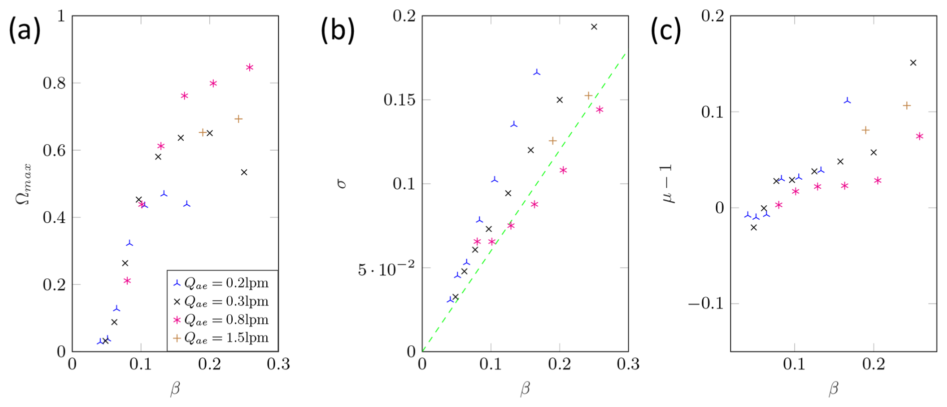
Figure E2 Measured transfer function parameters: maximum height (a), width (b), and shift (c) of the CDMA in DMA mode for d_p=200 nm.

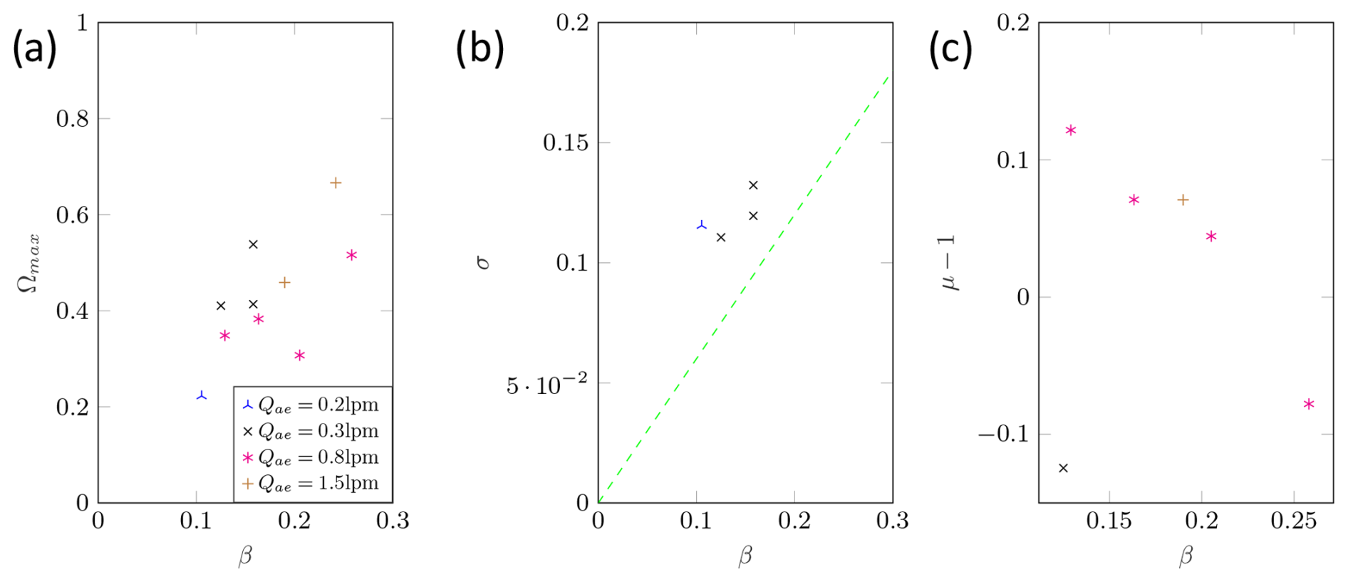
Figure E3 Measured transfer function parameters: maximum height (a), width (b), and shift (c) of the CDMA in AAC mode for d_p=50 nm.

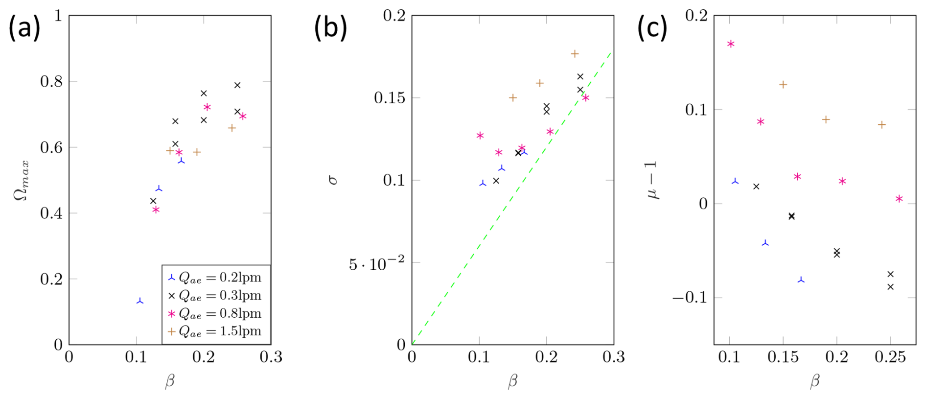
Figure E4 Measured transfer function parameters: maximum height (a), width (b), and shift (c) of the CDMA in AAC mode for d_p=200 nm.

Appendix F: Nomenclature

a,d	Fit parameters for the height of a Gaussian function	–
ac	Centrifugal acceleration	m s−2
c,e	Fit parameters for the width of a Gaussian function	–
Cu	Cunningham slip correction factor	–
c0	Total number concentration	# m−3
dm	Mobility-equivalent diameter	m
dae	Aerodynamically equivalent diameter	m
dst	Stokes equivalent diameter	m
dv	Volume-equivalent diameter	m
E	Electrical field magnitude	V m−1
Fc	Centrifugal force	N
Fel	Electrical force	N
FDr	Drag force	N
L	Length of the CDMA transfer path	m
mP	Particle mass	kg
n1	Particle number concentration after the first device in a tandem setup	# m−3
n2	Particle number concentration after both devices in a tandem setup	# m−3
Qa	Aerosol volume flow	m3 s−1
Qs	Sample volume flow	m3 s−1
Qsh	Sheath air volume flow	m3 s−1
Qex	Excess air volume flow	m3 s−1
QP	Particle charge	As
r1	Inner radius	m
r2	Maximum radius at which the particles enter	m
r3	Minimum radius at which the particles are still classified	m
r4	Outer radius	m
rin	Actual radius at which the particle enters	m
$\stackrel{\mathrm{‾}}{r}$	Average of the outer and inner radii	–
s	Radial distance	m
smax	Maximum radial distance	m
T	Truncation factor	–
u	Velocity of the air	m s−1
U	Voltage	V
wDr	Particle drift velocity	m s−1
$\stackrel{\mathrm{‾}}{x}$	Mean particle size	m
y	Position of the particle in the streamwise direction	m
Zp	Particle mobility	m2 (Vs)−1
Z∗	Nominal particle mobility	m2 (Vs)−1
$\stackrel{\mathrm{̃}}{Z}$	Normalized particle mobility	–
$\stackrel{\mathrm{̃}}{h}$	Ratio of the gap width to the mean radius	–

ρ	Particle density	kg m−3
β	Ratio of Qa to Qsh	−
η	Dynamic viscosity	Pas
κ	Ratio of r1 to r4	–
τ	Particle relaxation time	s
τ∗	Nominal particle relaxation time	s
$\stackrel{\mathrm{̃}}{\mathit{\tau }}$	Normalized particle relaxation time	–
$\stackrel{\mathrm{̃}}{{\mathit{\mu }}_{\mathrm{2}}},\stackrel{\mathrm{̃}}{{\mathit{\mu }}_{\mathrm{1}}}$	Fit parameters for the shift of a Gaussian function	–
$\stackrel{\mathrm{̃}}{\mathit{\mu }}$	Shift of the transfer function	–
Ωmax	Maximum height of the transfer function	–
σ	Width of the transfer function	–
ω	Angular speed	1 s−1
Ω	Transfer function	–