Measurements and modeling of urban secondary organic aerosol formation potential as a function of precursor volatility class in the Los Angeles area during summer 2022

Urban secondary organic aerosol (SOA) contributes to degraded air quality, which can affect human health. Improvements in Los Angeles (LA), CA, air quality have mainly plateaued since 2010. In summer 2022, measurements were made to quantify the SOA formation potential (SOA-FP) in ambient LA air. Two oxidation flow reactors (OFRs) ingested ambient air: one was equipped with an electrically conductive polymer inlet that denuded lower-volatility species, and the other was run without an inlet. This allowed the separate quantification of SOA-FP from higher- vs. lower-volatility precursors. To our knowledge these are the first direct measurements of these fractions. Measured ambient SOA was similar, and total SOA-FP was lower in 2022 vs. 2010, consistent with higher ambient OH causing greater consumptions of SOA precursors in 2022. The dual-OFR measurements suggest ∼ 31 % of the total SOA-FP is due to compounds with volatilities in the semi-volatile organic compound (SVOC) and lower intermediate-volatility organic compound (IVOC) ranges. Evidence suggests these lower-volatility precursors are mainly from direct emissions, rather than oxidation products from upwind aging. Results are compared to two box models: one based on CRACMM and the other adapted from a recent Caltech publication. CRACMM predicted ambient OA well but underpredicted SOA-FP by about a factor of 2, while the Caltech model underestimated OA and overpredicted SOA-FP by a factor of 2.5. Our study finds terpenoids contribute to, but do not dominate, SOA-FP.

1 Introduction

Aerosols are a major component of air pollution in urban areas around the world and contribute to reduced air quality, negative health effects in humans and animals, and decreased visibility (Founda et al., 2016; Losacco and Perillo, 2018; Shiraiwa et al., 2017). About 75 % of the fine-mode urban aerosol mass is organic, and a major fraction of that is secondary organic aerosol (SOA), formed from oxidation of gas-phase emissions (Hass-Mitchell et al., 2024).

The Los Angeles (LA) megacity in California has hosted many air quality field campaigns over the last few decades to better understand the area's atmospheric chemical processes and their evolution in time (Docherty et al., 2011; Hersey et al., 2011; Jensen et al., 2024; Ortega et al., 2016; Ryerson et al., 2013; Van Rooy et al., 2021). Since the 1950s, emissions reductions from mobile sources, outdoor burning and industrial processes have improved LA's historically poor air quality (Parrish et al., 2016). However, improvements in both ozone and organic aerosol (OA) have plateaued in the last decade (Kim et al., 2022; Nussbaumer and Cohen, 2021). Pollution sources such as volatile chemical products (VCPs) (McDonald et al., 2018) and cooking emissions (Hayes et al., 2015; Robinson et al., 2018; Zhu et al., 2025) continue to grow in relative importance. Knowledge of gas-phase pollutants with the highest contribution to SOA can help in understanding how to improve future air quality.

Oxidation flow reactors (OFRs) have been deployed around the world to study the relationship between gas-phase emissions and their SOA formation potential (SOA-FP) (Zhang et al., 2024a). OFRs are field-deployable reactors that can ingest and photochemically age ambient air. (Peng and Jimenez, 2020; Zhang et al., 2024a). SOA-FP is the amount of SOA that can be formed from the precursors present in air when they are reacted to completion with an oxidant. OFR studies have identified emissions from traffic, volatile chemical products, cooking and biogenics as sources of SOA-FP in urban areas (Hu et al., 2021; Liao et al., 2021; Liu et al., 2018, 2019a; Ortega et al., 2016; Saha et al., 2018; Shah et al., 2020; Tkacik et al., 2014; Zhang et al., 2024b). In urban settings, OFRs have demonstrated the high SOA-FP of ambient air at night (when precursor concentrations are high, and oxidants are low) and low SOA-FP of ambient air during the day (when precursors are being oxidized by the ambient photochemistry). At night, it is common for several micrograms per cubic meter of SOA to be produced in the OFR (Hu et al., 2021; Liu et al., 2019a; Ortega et al., 2016; Saha et al., 2018; Zhang et al., 2024b).

An OFR was deployed in LA in 2010 to measure the SOA-FP of ambient air (Ortega et al., 2016). Nighttime measurements showed an average of ∼ 5 µg m⁻³ of SOA-FP. Daytime OFR measurements collapsed onto the ambient measurements of SOA because the aging had already occurred outside, and no further SOA enhancements were formed in the OFR. Measurements in Beijing found similar diurnal trends for SOA, but with substantially higher SOA formation than in LA (∼ 10 µg m⁻³) due to higher precursor concentrations (Liu et al., 2018). Measurements in Pittsburgh and New York also show similar diurnal trends for SOA and found that nontraditional emission sources like VCPs are an important unaccounted source of urban precursors in SOA formation schemes (Shah et al., 2020).

When deployed in the field, OFRs typically ingest ambient air without any upstream separation techniques. The use of an inlet or inlet plate on the front of the OFR was qualitatively observed to result in reduced SOA formation, presumably from the loss of lower-volatility gas precursors, so OFRs are typically run with an open front end (Ortega et al., 2013). Therefore, the importance of different precursor groups to SOA-FP remains unknown. Laboratory work has allowed for quantification of the SOA-FP of key individual species, but this work is laborious, and there are thousands of individual species emitted in urban air. Recent studies modeling SOA formation in LA found contradictory results regarding the volatility range of the most important SOA precursors. For example, one model indicated that semi-volatile and intermediate-volatility organic compounds (S/IVOCs) were major contributors to SOA (Ma et al., 2017), while another suggested the opposite – that volatile organic compounds (VOCs) were dominant, and S/IVOCs were of very minor importance (Akherati et al., 2019). Additional experimental data could help evaluate model output to understand impacts on air quality.

In this work, we introduce a novel measurement technique to experimentally apportion SOA-FP in ambient air according to ambient VOC precursor volatility class. We demonstrate how low-cost tubing can be used as a “high-pass volatility filter” upstream of an OFR to separate ambient precursors into two volatility classes and measure the amount of SOA formed from each. We compare our results with predictions from a box model (Schulze et al., 2025) and the Community Regional Atmospheric Chemistry Multiphase Mechanism (CRACMM) (Pye et al., 2023).

2 Experimental

2.1 Campaign and measurement site

CalNexT 2022 was a measurement campaign designed to investigate urban VOC emissions and oxidation, ozone production, and aerosol formation (Jensen et al., 2024; Schulze et al., 2025). This campaign was a follow-up to the 2010 California Research at the Nexus of Air Quality and Climate Change (CalNex) campaign. To measure the well-mixed air of the Los Angeles Basin, we measured downwind of LA from as high a site as possible. A suite of state-of-the-art gas and aerosol instruments were installed in an air-conditioned penthouse on top of the tallest building at the California Institute of Technology (Caltech), which is also one of the tallest buildings in Pasadena. Inlets were placed out southwest-corner windows and also on the roof (∼ 40 m above the ground) of Caltech Hall (shown in Fig. 1). The measurements described here were conducted from 11 July to 14 August 2022. Winds were primarily from the southwest, putting the measurement site ∼ 3 h downwind of downtown LA in the afternoon (Washenfelder et al., 2011). During periods of transported wildfire smoke or biomass burning activity, we expect acetonitrile and OA to be correlated (Aiken et al., 2010; de Gouw et al., 2003). To understand if this campaign was influenced by wildfire smoke plumes or other biomass burning, we used the ambient acetonitrile measurements. The time series of acetonitrile in Fig. S1a in the Supplement shows some spikes, but these do not correlate with ambient OA or SOA-FP enhancements (Fig. S1c, d) and thus are likely from solvent use or other urban sources. We conclude that there is no significant biomass burning influence on this campaign data. Additionally, ambient temperatures (shown in Fig. S7c) were too high to expect local wood burning for warmth, as nighttime temperatures only dropped to ∼ 20 °C.

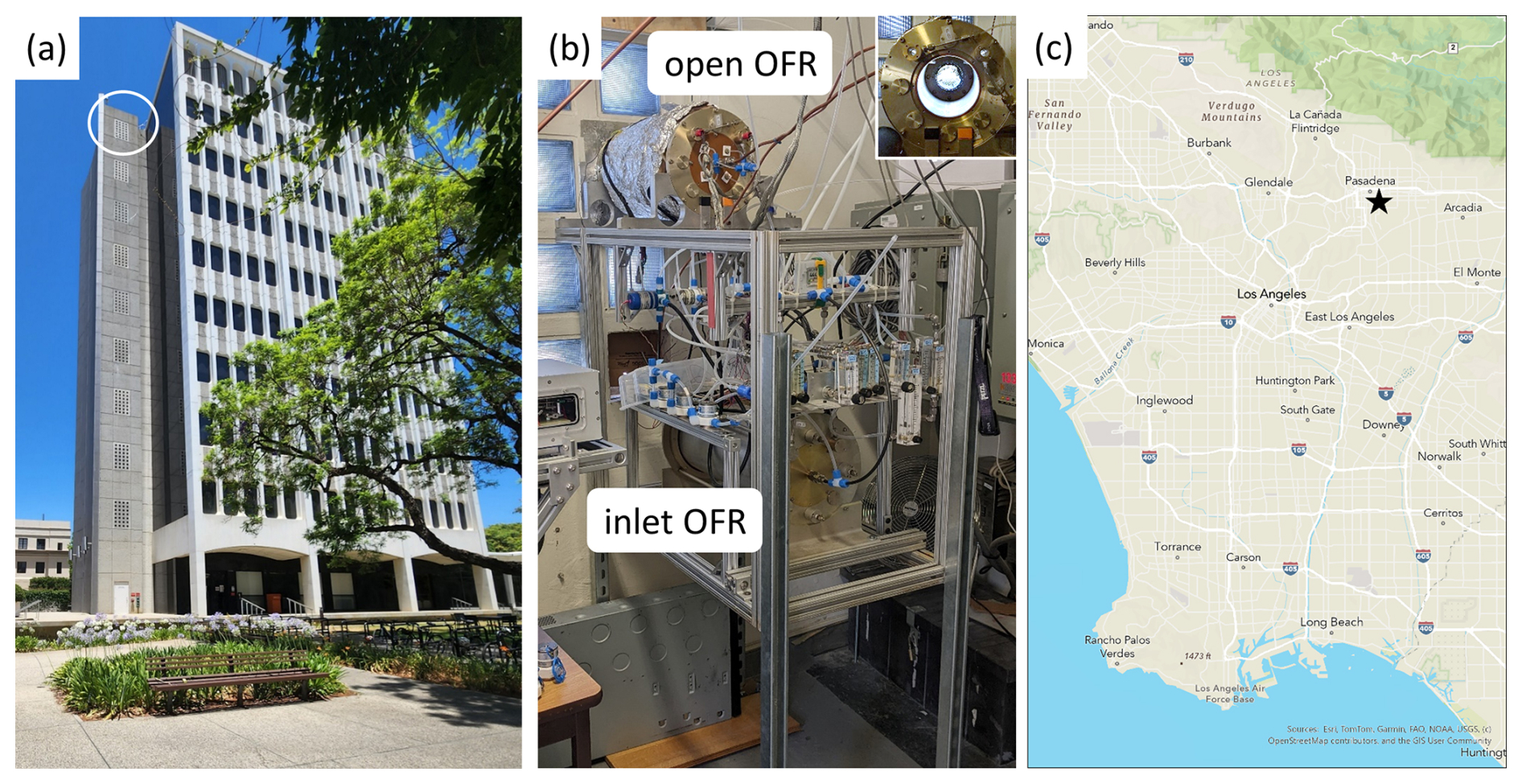
Figure 1 (a) A photo of Caltech Hall, where all instruments were located in a rooftop penthouse. Ambient inlets for the Vocus and inlet OFR were put out of the circled windows. The ambient inlet for the aerosol mass spectrometer (AMS) was located through a hole in the roof. (b) The dual-OFR system was mounted against the windows. The top “open” OFR sampled ambient air through an open window without an inlet, and the bottom “inlet” OFR sampled ambient air through a tubing inlet. The inset shows a photo of the top OFR when open for servicing. For more details about the open OFR, see Fig. S2. (c) A map of the campaign location, with a star indicating the sampling site at Caltech, which was ∼ 3 h downwind of LA. The base map was designed and developed by Esri, TomTom, FAO and USGS | Powered by Esri.

2.2 Dual-OFR system

Two potential aerosol mass oxidation flow reactors (OFRs) were used to simulate photochemical aging of ambient air (Fig. 1b). OFRs are cylindrical 13.1 L aluminum reactors that simulate atmospheric aging on a short (∼ 3 min) timescale (Kang et al., 2007). They have been used in many studies to investigate atmospheric processes in urban areas (Hu et al., 2021; Liao et al., 2021; Liu et al., 2018, 2019a; Ortega et al., 2016; Saha et al., 2018; Shah et al., 2020; Tkacik et al., 2014; Zhang et al., 2024b). A list of OFR configuration details is included in Table S2.

Both of the OFRs deployed in this study were manufactured by Penn State University and run in OFR185 mode (Peng and Jimenez, 2020). In this mode, two Teflon-sleeved, low-pressure mercury lamps (model no. 82-9304-03, BHK Inc., Ontario, CA) with discrete emission peaks at 185 and 254 nm photolyze water and ozone inside the OFR to generate hydroxyl (OH) radicals. A steady flow (∼ 30 cm³ min⁻¹) of nitrogen passed through each Teflon lamp sleeve to cool and protect the lamps. No ozone was injected into the OFRs. While both OH radicals and ozone are formed in the OFR, the ratio of OH to ozone exposure is ∼ 100 times larger than in the atmosphere (at the surface). Even for species like limonene that react quickly with ozone, OH chemistry is dominant in the OFR (Peng et al., 2016; Peng and Jimenez, 2020). Since the midday photochemical age of ambient air was 0.5 d (as discussed in Sect. 3.4), and the OFRs were achieving an additional 2 d of aging in a 3 min residence time, we estimate that the concentration of OH radicals in the OFR was ∼ 240 times that of ambient air. The rapid consumption of NO_x leads to low-NO conditions in the reactor (Peng and Jimenez, 2017). As discussed in Peng and Jimenez (2020), in order to maintain atmospheric relevance under low-NO conditions, OFRs need to be tuned carefully. OH concentrations should be high enough to minimize non-tropospheric VOC photolysis, but low enough so that fast autoxidation reactions can occur. In this work we targeted an OH exposure of ∼ 2 equivalent days to exhaust SOA precursors and measure the full SOA-FP of ambient air (Hayes et al., 2015; Ortega et al., 2016). Fast autoxidation reactions are still competitive at this level of exposure, while slower ones have reduced importance compared to ambient conditions (Peng et al., 2019). This exposure, along with the humidity of ambient air and the estimated total external OH reactivity of 20 s⁻¹, puts the OFR in “safe” operating conditions (Peng and Jimenez, 2020). In a previous campaign, the SOA yields in the OFR for several terpene species were probed using standard addition and found to be comparable to those of low-NO_x chamber studies (Palm et al., 2018). Given the state of the knowledge about ambient SOA-FP, oxidation mechanisms and oxidation conditions, it is still unclear whether other deviations between average OFR oxidation conditions and average ambient conditions could bias the experimental VOC-to-S/IVOC SOA-FP apportioning. The OFR lamps were turned off for 40 min every 6 h to quantify ambient gas and aerosol transmission in the absence of oxidation.

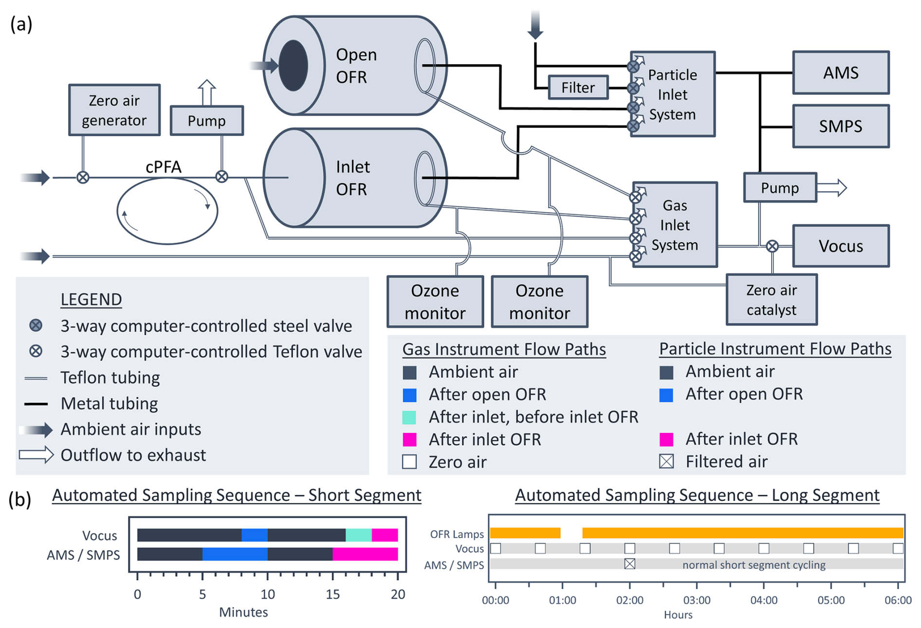
Figure 2 (a) A schematic of the sampling setup for the campaign. The instruments switched between sampling ambient air, O-OFR, I-OFR and zero air. The Vocus also sampled after the I-OFR inlet but before the I-OFR to characterize gas transmission through the inlet. Flow paths for aerosol measurements always went through metal tubing (or cPFA tubing in the case of the inlet OFR). Flow paths for gas measurements always went through PFA Teflon tubing. The inlet for the I-OFR had a zero-air generator plumbed on the front, which flowed zero air into the inlet to an exhaust pump when other inlets were in use. The inlet system could switch between four different denuding inlets, but only one was used throughout the campaign, so only one is shown here for clarity. (b) A schematic of the automated sampling sequences. The short segment repeated every 20 min. Once every 6 h, the lamps in the OFRs were turned off. The AMS and SMPS sampled filtered air on an offset 6 h schedule. The Vocus spent 2 min sampling zero air every 40 min.

A schematic of the dual-OFR system is shown in Fig. 2a. The open OFR (O-OFR hereafter) was run without an inlet or front plate so that all gas-phase precursors entered the OFR. The OFR opening was 14 cm wide and had a coated (Sulfinert coating by SilcoTek, Bellefonte, PA) coarse mesh screen (1 mm squares) to prevent debris and insects from entering the OFR and to break up wind eddies. The O-OFR was housed inside the penthouse and was situated against an opening where a window was removed. To reduce building effects and prevent room air from being sampled, the O-OFR was attached to a metal cone that extended outside through the brick wall and was sealed from room air with aluminum tape. The cone had a tapered diameter (12.5 cm at the OFR down to 9.5 cm) and was 27 cm long; it protruded ∼ 10 cm out from the exterior wall of the building. A custom-built exhaust system pumped away air at the cone's edges to avoid sampling gases that had undergone gas–wall interactions. More details and photos are shown in Fig. S2.

New to this work, a conductive polymer inlet was installed on the second OFR (inlet OFR, hereafter I-OFR), which denuded lower-volatility precursors from the ambient gas stream. Electrical conductivity is important for high particle transmission. It is well known that polymer tubes absorb gas-phase species and that this process is chromatographic in nature, reversible and independent of compound concentration (Deming et al., 2019; Liu et al., 2019b; Morris et al., 2024; Pagonis et al., 2017). These interactions can have (i) negligible effects on gas transmission, (ii) cause significant delays, or (iii) denude species completely depending on the volatility of the species and the properties of the tubing material. The absorptive capacity of the tubing used here ($\mathrm{1}/\mathrm{4}$ in. OD electrically conductive perfluoroalkoxy alkane (cPFA) Teflon, ∼ 3.5 m, Fluorostore, part no. FO152O2G, Parsippany, NJ) has been experimentally characterized in previous work (Morris et al., 2024).

The gas volatility separator designed and described by Morris et al. (2024) is an inlet system capable of switching between four different inlets automatically. It was attached to the I-OFR using a standard OFR front plate with a custom coated (Sulfinert coating by SilcoTek, Bellefonte, PA) inlet piece for radial, rather than jet, flow; the details of this piece are shown in Nault et al. (2018), specifically their Fig. S13. A zero-air generator (Thermo Scientific, Model 1160, Waltham, MA) was plumbed to three-way Teflon solenoid valves (Cole-Parmer, part no. EW-01540-18, Vernon Hills, IL) at the front of each inlet. When the inlets were not being used to direct ambient air to the I-OFR, they were flushed with zero air. This allowed the VOCs from ambient air to depassivate from the inlets so that the denuding properties would remain constant in time. Due to issues with VOC emissions or similarity in gas transmission of the other inlet materials, only the cPFA inlet was used extensively. This is discussed in more detail in Sect. 3.10.

The output plumbing was the same for each OFR. It is critical to have an all-Teflon pathway for the highest gas transmission and an all-metal pathway for the highest aerosol transmission, as each is lost to the other material type (Deming et al., 2019). Each OFR had a metal center port that was used to draw 2 L min⁻¹ to the aerosol-phase instruments (passing through a $\mathrm{1}/\mathrm{4}$ in. OD 2.5 m long copper tube) and a Teflon ring port that was used to draw 2.4 L min⁻¹ to the gas-phase instruments (passing through a $\mathrm{1}/\mathrm{4}$ in. OD 1 m long PFA tube). The total flow through each OFR was 4.4 L min⁻¹; given an internal volume of 13.1 L, the residence time of ambient air inside the OFRs was ∼ 3.0 min.

2.3 Online instrumentation

A high-resolution time-of-flight aerosol mass spectrometer (AMS) (Canagaratna et al., 2007; DeCarlo et al., 2006) was operated by Caltech and used to monitor chemical composition of non-refractory submicron aerosol with 1 min resolution. Schulze et al. (2025) provide a detailed summary of the AMS sampling setup and ambient data and compare the results with those from the 2010 and 2020 campaigns (Schulze et al., 2025). The instrument was run in “V mode”. Sensitivity calibrations were made approximately weekly using dry ammonium nitrate and ammonium sulfate aerosols. A scanning mobility particle sizer (SMPS) with a condensation particle counter (TSI, Model 3775, Shoreview, MN), differential mobility analyzer (TSI, Model 3081) and classifier (TSI, Model 3080) quantified the size distribution of measured aerosols with 2.5 min resolution, always sampling the same air as the AMS. The time series of the SMPS size distribution is shown in Fig. S3a. The average size distribution is shown in Fig. S3b. Schulze et al. (2025) report a regression slope of 1.03 between the AMS and SMPS particle volume for this campaign.

A Vocus-2R proton-transfer-reaction time-of-flight mass spectrometer (Krechmer et al., 2018) (Tofwerk AG and Aerodyne Research, Inc.), hereafter referred to as the Vocus, was used to measure concentrations of gas-phase species with 1 sec resolution. Jensen et al. (2024) provide a summary of the ambient Vocus data during the campaign and compare the data to 2010 measurements. The instrument was calibrated with a 13 VOC standard mixture using two methods: a manual multipoint calibration was performed daily, and the instrument also sampled a single dilution of the standard mixture for short periods every 80 min throughout the day. More details about the instrument and data processing can be found in Jensen et al. (2024).

The aerosol-phase instruments sampled one of four pathways at any given time, which were ambient air, the output of the O-OFR, the output of the I-OFR or HEPA-filtered ambient air to zero the instruments. To control which pathway the aerosol-phase instruments were sampling, a series of automated three-way stainless steel valves (43 series, Aerodyne Research Inc., Billerica, MA) directed flow, automated by custom acquisition software (programmed with the Multi-Instrument Control and Acquisition System (MICAS), Original Code, Boulder, CO) within Labview. When the pathways were not being sampled by the instrumentation, vacuum lines on the three-way valves pulled an equivalent amount of flow to ensure the flow rate through the OFRs and inlets stayed constant. Figure 2b shows a schematic of the automated sampling sequence used for most of the campaign. The aerosol-phase instruments sampled each pathway for 5 min at a time.

The Vocus sampled one of five pathways at any given time, which were ambient air, the output of the O-OFR, the output of the I-OFR, the input of the I-OFR (after the inlet) or ambient air passed through a heated catalytic zero-air generator (Tofwerk AG, Thun, Switzerland) to zero the instrument. To control which pathway the gas-phase instruments were sampling, a series of three-way Teflon solenoid valves (Cole-Parmer, part no. EW-01540-18, Vernon Hills, IL; NResearch Inc., part no. 648T032, West Caldwell, NJ) directed flow, automated by the same acquisition software. When the pathways were not being sampled by the instrumentation, vacuum lines on the three-way valves pulled an equivalent amount of flow to ensure the flow rate through the OFRs and inlets stayed constant. The Vocus sampled each pathway for 2–8 min, depending on the sequence, shown in Fig. 2b.

Several carbon dioxide (CO₂) instruments were used to leak check the sampling system, with CO₂ being used as a tracer of opportunity, since it was elevated in the penthouse due to human breath. One CO₂ sensor (Aranet, Aranet4 HOME, Aurora, CO) was used to monitor CO₂ inside the penthouse, a second CO₂ analyzer (LICOR, 840A, Lincoln, NE) was used to measure CO₂ inside the open OFR, and a third CO₂ sensor (Teledyne, M300U2, Thousand Oaks, CA) was used to measure ambient CO₂ levels from the roof.

2.4 Estimation of OH exposure in the OFRs

OH exposure is a measure of OH radical concentrations integrated over time for a given air mass. Coupled with a reference average 24 h atmospheric concentration of OH radical (1.5 × 10⁶ molec. cm⁻³) (Mao et al., 2009), OH exposures can be translated into photochemical ages, in days, and are then comparable to atmospheric aging outdoors.

During the campaign, OH exposures were estimated with an equation from Li et al. (2015) based on a parameterization of the ratios of $\mathrm{254}/\mathrm{185}$ nm light flux, OFR ozone concentrations, OFR water concentrations and an estimate for OH reactivity. We used a default OH reactivity value of 20 s⁻¹ for urban air (Yang, 2023). This method is particularly useful in operations planning and for tracking real-time changes in OH exposure in the field but typically only estimates the photochemical age to within a factor of 2–3. The lamp powers were tuned so that both OFRs targeted a photochemical age of ∼ 2 d of equivalent exposure. Two ozone monitors (2B Technologies, Model 205, Broomfield, CO; Thermo Electron Corp., Model 49i, Waltham, MA) were used to measure ozone exiting each of the OFRs. More details on calibration of the ozone measurements and associated discussion can be found in Fig. S4.

During post-campaign analysis, the real-time measurements of toluene decay in the OFRs during the campaign were used to calculate final OH exposure estimates. Toluene has been shown to have only a minor (< 5 %) possible interference from fragmentation of oxidation products when measured with the Vocus in an urban area (Coggon et al., 2024b). In the 3 min residence time of the OFRs toluene is expected to decay significantly, but not completely. The first-order rate coefficient constant for reaction with OH radicals (5.63 × 10⁻¹² cm³ molec.⁻¹ s⁻¹ at 298 K) (Atkinson and Arey, 2003a) was used to convert the observed percent decay (relative to ambient toluene concentrations) into an OH exposure estimate for each OFR. Comparisons of the two methods are shown in Sect. 3.4.

2.5 Offline analysis to estimate volatility transmission cutoff for I-OFR

Since the Vocus can only measure partially into the upper IVOC region, the Vocus data alone are not sufficient to determine the volatility cutoff of the inlet. To overcome this limitation, ambient LA air was sampled onto sorbent cartridges in a separate system for offline lower-volatility species analysis. Sorbent cartridge collection largely followed the protocols described in Tasnia et al. (2026). In brief, dual sorbent bed (100 mg Tenax TA 35/60 and 200 mg Carbograph 1 TD 60/80 in series) co-located cartridge samples were taken with and without a non-conductive polytetrafluoroethylene (PTFE) inlet (∼ 1.5 m length, $\mathrm{1}/\mathrm{4}$ in. OD) three times a day for 3 d, resulting in nine paired samples. Samples were collected at 05:30, 09:00 and 14:00 PDT for a duration of 1 h at a flow rate of ∼ 250 cm³. A PTFE filter (Millipore, part no. LSWP04700) was placed upstream of all sorbent cartridges to remove particulate matter. Although the offline setup had a different inlet material, Morris et al. (2024) show that non-conductive PTFE and conductive PFA (used as the I-OFR inlet) have similar absorptive capacities; therefore the absorption kinetics of the offline setup have been deemed a suitable proxy to estimate the volatility transmission curve for the I-OFR. We have run simulations of VOC transmission through both inlets using the model published in Pagonis et al. (2017), which are included in Fig. S5. The PTFE inlet is predicted to have a similar species transmission curve vs. volatility (C^∗) compared to the cPFA inlet (within an order-of–magnitude in C^∗). This does not include the sorption caused by the PTFE filter in the offline system or by the valves in the I-OFR sampling system, which are both expected to increase denuding.

The cartridges were transported to the University of California, Riverside, and analyzed using a Turbomatrix 650 automated thermal desorption (ATD) system (PerkinElmer, Waltham, MA) coupled to a Pegasus 4D GC × GC-TOF-MS (LECO Corp., St. Joseph, MI). The sorbent cartridge samples were run following the analytical procedures of Hatch et al. (2019), with modifications to the column set and temperature ramp to capture lower-volatility compounds. The modified column set was a Rxi-5MS (30 m, 0.25 mm i.d., 0.25 µm film thickness) primary column and Rxi-17SilMS (1.5 m, 0.15 mm i.d., 0.15 µm film thickness) secondary column. Before analyzing the cartridges, a gaseous internal standard mixture of toluene-d8, 1-bromo-4-fluorobenzene and 1,2-dichlorobenzene was automatically injected using the ATD. Then the cartridges were desorbed at 350 °C, and 13 % of the sampled mass was transferred to GC × GC-TOF-MS. The mass spectra acquisition rate was 50 Hz. The modified temperature ramp is shown in Fig. S6.

To confirm that the modified analytical procedures successfully allowed detection of lower-volatility compounds, a C₇–C₄₀ saturated alkanes standard (Sigma Aldrich, Burlington, MA) diluted to 40 ng µ L⁻¹ and 1 µL was spiked onto a sorbent tube. The sorbent tube was analyzed using the same GC and MS methods as noted above. Octacosane (C₂₈H₅₈, C^∗ at 298 K = 1.5 µg m⁻³) was the highest-molecular-weight alkane detected in the chromatograms.

2.6 Modeling

2.6.1 Caltech box model

We used a box model developed and described by Schulze et al. (2025) to simulate ambient OA as well as the aged OA formed in both OFRs. The model is conceptually built on previously developed frameworks and parameterizations for urban air quality modeling (Dzepina et al., 2009; Hayes et al., 2015; Ma et al., 2017; Pennington et al., 2021). In brief, the model requires measured background-corrected carbon monoxide (ΔCO) to scale normalized emission estimates for on-road, non-road and area/stationary sources in LA for 2022 to initialize the precursor concentrations. Emissions are then lumped according to their volatility (C^∗) and source and are oxidized until the experimentally determined photochemical age (for each of ambient air, O-OFR or I-OFR) has been reached. Species partition according to their C^∗ values to form OA.

Biogenics (isoprene and monoterpenes) are treated separately in the model. Schulze et al. (2025) use a simplified Lagrangian method to estimate biogenic SOA; more details can be found in their Sect. S5.2.7. In brief, the model uses back trajectories to integrate the amount of SOA formed from isoprene and monoterpene oxidation for each hour of the diurnal cycle. They assume a mass yield of 5 % for isoprene and 20 % for terpenes. The integrated amount of SOA is added to the total modeled OA at the end of the simulation. This calculation of the biogenic contribution to ambient SOA (before the OFR) was kept the same in our simulations. Since this method does not do gas-phase accounting, it would not work to simulate the SOA-FP in the OFR of biogenics that are in the gas-phase under ambient conditions. Therefore, we adapted the Caltech model to perform this aging. We initialized the biogenic concentration of ambient gas-phase monoterpenes as half the measured concentration of monoterpenes using the Vocus. We assume the other half of the measured monoterpenes come from anthropogenic sources (Katz et al., 2025; Tasnia et al., 2026) and are therefore already accounted for by the VCP emissions in the model. We use the same mechanism already existing in the model for aging of terpenes from VCPs.

To simulate the O-OFR, the model was run without changes until the photochemical age reached ambient levels. Then the air was aged further without dilution until the experimentally determined O-OFR photochemical age was reached. To simulate the I-OFR, the same process was used, but the precursor concentrations were adjusted (decreased or kept constant, depending on their C^∗) to reflect the measured transmission curve determined in Sect. 3.1. Then the model was run until the experimental photochemical age of the I-OFR was reached.

The model outputs diurnals of POA and SOA, which we sum in our analysis to compare total OA between the model and measurements in Sect. 3.5. We also investigate the total OA apportioning according to emission source and volatility.

2.6.2 Community Regional Atmospheric Chemistry Multiphase Mechanism (CRACMM)

The Community Multiscale Air Quality Monitoring System (CMAQ, Version 5.5) is a three-dimensional air quality forecasting model, developed and maintained by the US Environmental Protection Agency (EPA) (US EPA Office of Research and Development, 2024). The CMAQ system uses Weather Research Forecasting (WRF) meteorology and chemically speciated emissions for 2019 informed by the National Emission Inventory (NEI; U.S. Environmental Protection Agency, 2026) and methods within CMAQ (US EPA, date of release: 2025). The emissions react and are transported in the model to predict ambient pollutant concentrations across a specified area. Within CMAQ chemistry is parameterized, in this work, by the Community Regional Atmospheric Chemistry Multiphase Mechanism (CRACMM) (Pye et al., 2023) version 2 (Skipper et al., 2024). In brief, CRACMM uses ∼ 500 reactions that involve over 200 gas- and aerosol-phase species to predict atmospheric transformations of organic and inorganic species, as well as ozone and OA concentrations. The mechanism contains both explicit and lumped reactions, with many reactive organic carbon species lumped by C^∗ and chemical functionality (degree of oxygenation and aromaticity). Oxidation occurs through reaction with various oxidants (OH radicals, NO₃ radicals, ozone, etc.) as well as pathways such as photolysis, autoxidation and heterogeneous chemistry to form products. Gas–aerosol partitioning occurs for a subset of species (those with C^∗ < 1000 µg m⁻³) which contribute to the growth of OA in the model. Hourly CMAQ output of all chemical species as well as meteorological parameters for LA (34.136866° N, 118.126099° W) were extracted from the CMAQ results of Skipper et al. (2024) from 11 July 2019 to 14 August 2019 for comparison with 2022 ambient measurements (Sect. 3.5).

To simulate the amount of OA in the OFRs, which perform additional aging on top of ambient aging, we ran CRACMM2 independently of CMAQ as well. The full mechanism was used, excluding photolysis and heterogeneous reactions. In addition, reaction R114a (a large organic peroxide reaction with OH) was removed due to duplication (with reaction ROCOXY16c), consistent with CRACMM version 3. The mechanism was imported into a kinetic solver (KinSim, Version 4.21) (Peng and Jimenez, 2019). The KinSim output of an example chamber simulation was compared with the same simulation performed in F0AM and found to be identical within computer numerical precision. CRACMM was then merged with an existing OFR-specific mechanism (Peng and Jimenez, 2020). The OFR-specific mechanism produces oxidants from input photon fluxes (at 185 and 254 nm). Before the merge, we tuned the input photon flux parameters so that the photochemical age and ozone concentrations best represented our experimental values while keeping the $\mathrm{254}/\mathrm{185}$ ratio consistent with Li et al. (2015).

To initialize the diurnal CRACMM simulations, CMAQ model output for LA from 11 July to 14 August 2019 was averaged into diurnal cycles. This was the closest year to 2022 for which CMAQ output was available, so key CMAQ outputs were compared to measurements in Fig. S7. Temperature, ozone, CO and NO_x (NO + NO₂) showed very close agreement between the 2019 CMAQ output and 2022 measurements, indicating the meteorology and magnitude of urban emissions were comparable between the two years. Comparisons of gas-phase precursors showed varied results. Some species (including sesquiterpenes, acrolein, isoprene and styrene) were underestimated by CMAQ compared to the measurements. Other species (including aromatics, toluene, benzene and monoterpenes) were overestimated by CMAQ compared to the measurements. Key VOCs were adjusted using Vocus measurements from 2022. Section S1 details how the constraints were used to make these adjustments, and Table S3 lists the constraints by CRACMM species. By constraining these species with the Vocus measurements, we are able to better evaluate CRACMM as a chemical mechanism rather than the accuracy of the CMAQ output.

The O-OFR was simulated by allowing oxidation and partitioning to occur until the experimentally determined OFR photochemical age was reached. The I-OFR was run in the same way as the O-OFR, but to initialize the I-OFR simulation the precursor concentrations were adjusted to reflect the measured transmission curve determined in Sect. 3.1. The reported simplified molecular input line entry system (SMILES) was put through the SIMPOL (Pankow and Asher, 2008) parameterization for volatility estimation to calculate a C^∗ value for each species.

3 Results and discussion

The results section contains the following topics: (i) a description of the volatility cutoff for the inlet on the I-OFR, (ii) quantification of total OA and SOA-FP through the different sampling pathways, (iii) detailed specifics on the corrections of the measurements, (iv) modeling results, (v) modeling sensitivity testing, (vi) correlation analysis of measured SOA-FP with measured VOCs, and (vii) a discussion of the importance of terpenes in regard to SOA-FP.

3.1 Characterizing inlet transmission of gases

3.1.1 Using Vocus measurements to determine inlet volatility cutoff

As seen in the sampling sequence (Fig. 2b), measurements were made before and after the cPFA inlet of the I-OFR in order to characterize transmission of gases. All species detectable with the Vocus were transmitted close to 100 % through the inlet. This includes dimethylnaphthalene and C₁₂ aromatics, which have SIMPOL (Pankow and Asher, 2008) volatility estimates on the order of 10⁵ µg m⁻³. Figure 3a shows the measured transmission for selected species, while Fig. S8 shows the transmission of all measured gases.

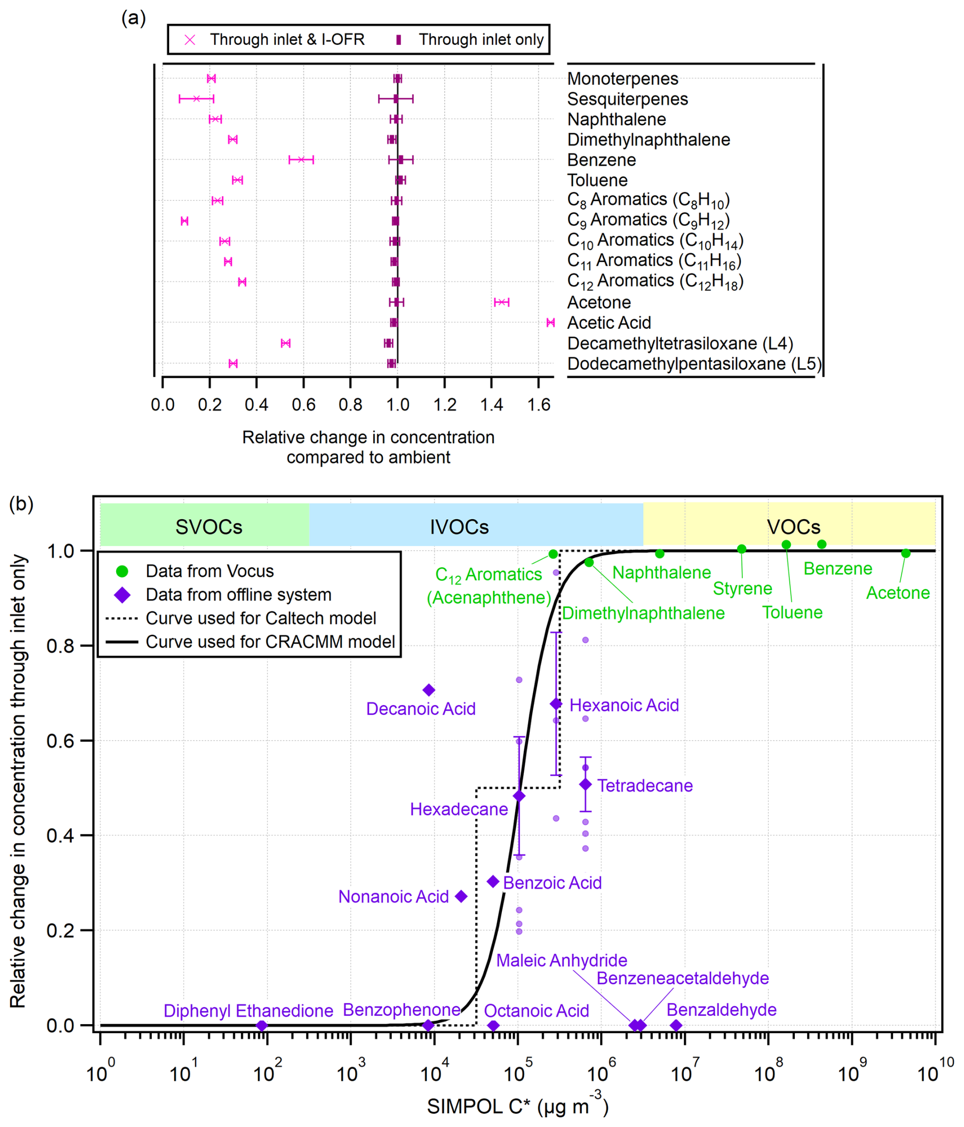
Figure 3 (a) Measured relative change in concentration, compared to ambient, through the inlet (but before entering the OFR) and through the inlet and the I-OFR. When passing through the I-OFR, some species decrease due to oxidation, while others increase since they are formed as oxidation products. A subset of species measured by the Vocus are shown here; the full list is shown in Fig. S8. The species are sorted by chemical category and then by increasing OH rate coefficient top to bottom. Error bars represent 1 standard deviation. (b) Relative change in concentration, compared to ambient, through the inlet (without active OFR) vs. SIMPOL volatility estimates for both the online and offline datasets. The lowest-volatility VOCs measured by the Vocus were dimethylnaphthalene and C₁₂ aromatics, which were transmitted without significant losses through the inlet. C₁₂ aromatics are not speciated in the Vocus, so we estimated the volatility using acenaphthene as a proxy. The offline data are shown with both individual data points (light-purple circles) and darker symbols with error bars with the standard error of the mean (for species that were detected in more than one sample). The transmission curve used for the inlet in both models was fit to all data except benzaldehyde, benzeneacetaldehyde and maleic anhydride, which we believe are decomposition artifacts.

In addition to the transmission through the inlet, we have also plotted the average relative change in concentration for species after the inlet and I-OFR, which includes changes due to chemical reactions in the OFR. Precursor species, like toluene and C₈ aromatics, react with OH radicals and therefore have depleted concentrations after the OFRs. Reaction of these precursors leads to oxidized product formation. Species with a strong secondary source, like acetone and acetic acid, have enhanced concentrations in the OFR. For functional group series, like C_8–12 aromatics, typically species with increasing carbon numbers react faster with OH so that lower-volatility species react away to a larger extent during the OFR residence time. C_6–9 aromatics follow this trend in Fig. 3a. However the trend is unclear for C_9–12 aromatics. This may be due to the decreasing signal-to-noise ratio in the Vocus measurements with increasing mass-to-charge ratio, as the relative change in concentration compared to ambient is highly dependent on the instrument zeros. In addition, de Gouw et al. (2017) have shown that the rate coefficient with OH radicals for grouped species such as C_x aromatics may not be monotonic and may change in time as the actual mix of species in ambient air varies.

3.1.2 Using offline analysis of filters to estimate inlet volatility cutoff

A separate setup where gases were sampled with and without inlet tubing, followed by offline analysis, was used to provide information about precursor transmission for lower-volatility species (see Sect. 2.5 for methods and setup). Although the offline setup had a different inlet tubing material, Morris et al. (2024) have shown that non-conductive PTFE (used as the offline setup inlet) and conductive PFA (used as the I-OFR inlet) have very similar absorptive capacities. Therefore the absorption kinetics of the offline setup have been deemed a suitable proxy for the inlet of the I-OFR.

The relative change in concentration was calculated by dividing the signal seen for the cartridges sampled through the non-conductive PTFE inlet by the signal seen for the inlet-less cartridges. Figure 3b shows the fraction transmission of all measured species according to their SIMPOL C^∗ estimates (Pankow and Asher, 2008). Standard errors were calculated for several species with more than one data point and are included in Fig. 3b. Data points with a transmission of zero indicate species detected only in the samples without an inlet. These include a few higher-volatility species, like benzaldehyde. While benzaldehyde is not directly reported in this study (due to lack of a standard), species of this volatility are expected to be fully transmitted with and without the inlet. The most likely explanation for the appearance of these higher-volatility species in samples without the inlet is that the high-temperature ramp (up to 280 °C) of the GC column led to thermal decomposition of larger, lower-volatility species that were captured in the inlet-less samples. The smaller thermal decomposition products were not detected in the samples with an inlet, since the larger, lower-volatility samples were not transmitted. Benzaldehyde has been shown to be a thermal decomposition product of aromatic flavoring compounds in vaping literature under the same temperature range used here, further supporting this idea (Blazsó et al., 2018; Chen et al., 2021).

We estimate that the inlet of the I-OFR is only transmitting VOCs and the most volatile ∼ $\mathrm{1}/\mathrm{3}$ of IVOCs. Transmission curves used for both models are shown in Fig. 3b. To determine the curve, we first obtained an estimate of the shape of the transmission curve. For this purpose we ran a simulation using a previously published tubing model described in Pagonis et al. (2017) that compared well with experimental data. We determine the shape of the transmission curve by fitting the Hill equation to the model results vs. C^∗. We then allowed the Hill curve to move left or right in log (C^∗). The best position of the curve was obtained by orthogonal distance regression. Since CRACMM is at least partially speciated and includes representative structures for all mechanism species, we used the Hill equation to translate C^∗ values of each species into fractional transmissions. For the Caltech model, the same curve was applied but described per volatility bin.

Papers that have studied oxygenated organics in Teflon sampling lines and chamber walls (Krechmer et al., 2016; Pagonis et al., 2017; Huang et al., 2018; Deming et al., 2019; Liu et al., 2019b) found that species with oxygenated functional groups partitioned to surfaces less efficiently than species without oxygen (for the same saturation concentration). This is likely due to an increased activity coefficient compared to non-oxygenated species (Krechmer et al., 2016; Huang et al., 2018). Therefore, the transmission of moderate-volatility oxygenated species could be underestimated in this work, since we predicted inlet transmission based on volatility alone. However, in this study the SVOCs that are SOA precursors may be primarily emitted or lightly oxidized and thus may not have such high activity coefficients on Teflon. We do not see evidence of higher-than-expected transmission of low-volatility species in Fig. 3b; the final transmission curve appears to fit all the data.

3.2 SOA formation potential (SOA-FP) measurement

Throughout the campaign the instruments sampled ambient air, the O-OFR and the I-OFR, switching every few minutes according to the sequences in Fig. 2b. Figure 4 shows a brief time series of several key gas-phase species sampled through the three pathways by the Vocus. As expected, oxidation products had enhanced concentrations (above ambient) during the OFR measurement periods, while precursor gas species decayed during OFR periods. Note that the corrections described later in Sect. 3.3 have been applied to these data. Typically we would report any corrections first, but since the dual-OFR technique is both new and complex, we present the data first to ground readers before discussing details.

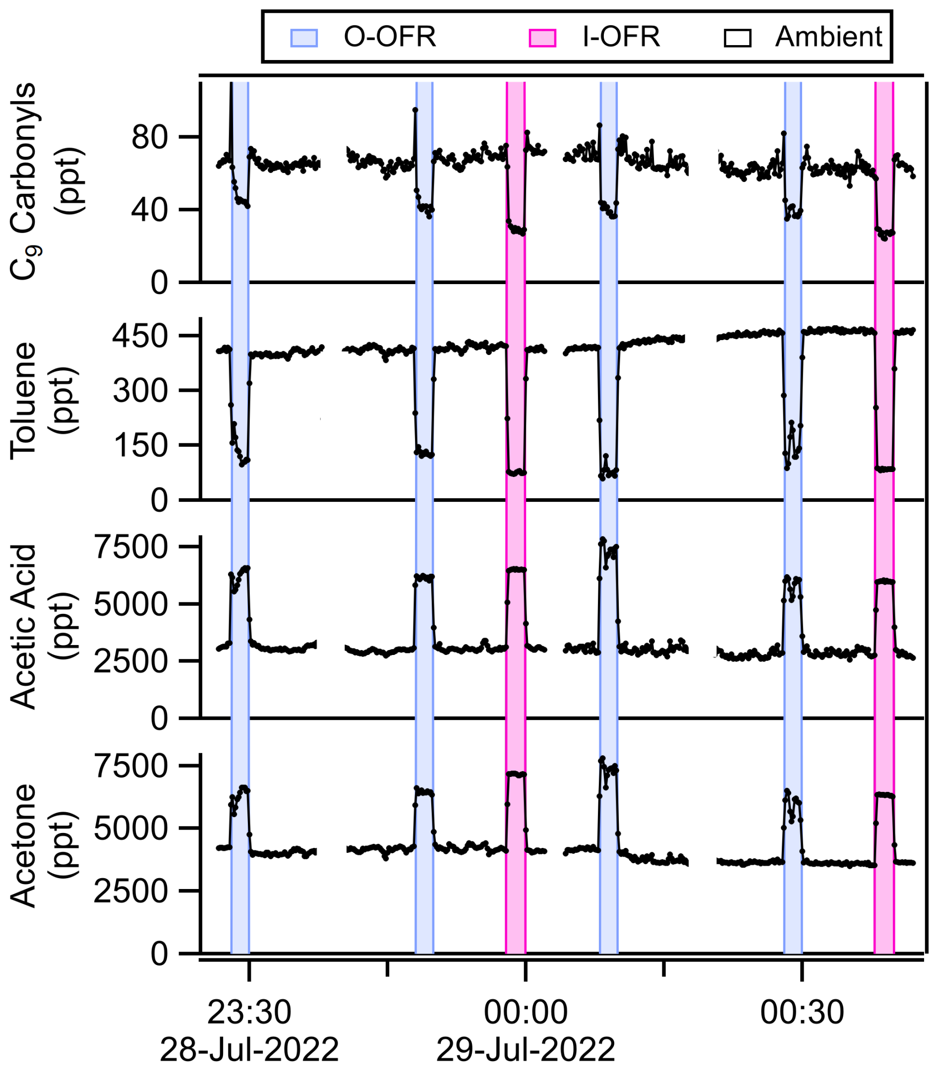
Figure 4 A representative night time series of four gas species as measured by the Vocus through the different sampling pathways. Species formed in the OFRs as oxidation products (acetone and acetic acid for example) show enhancements above ambient, while precursor species (C₉ carbonyls and toluene for example) show decays during the OFR periods.

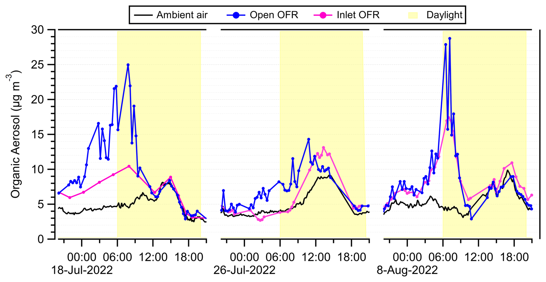
Figure 5 Time series of measured OA during 3 representative days for ambient air, the O-OFR and the I-OFR. Daylight hours are shown in shaded yellow.

The measured OA is shown through each pathway for 3 representative days in Fig. 5. There was limited day-to-day variability in the temperature and amounts of ozone, NO_x and CO, as seen in Fig. S7c. There was also limited variability in ambient and OFR OA, as shown in Fig. 6a. The ambient OA peaked in the afternoon; this was expected because ambient aerosol formation requires sunlight for initiation and is delayed due to transport of emissions from downtown LA (Hayes et al., 2013). The OFR OA peaked in the morning, when photochemistry was not active, and precursor concentrations were at their highest. High precursor concentrations react with OH radicals in the OFRs to initiate aerosol formation. By the afternoon, data from both OFRs collapsed onto the ambient measurements. This indicates that ambient air had effectively run out of SOA-forming precursors, since no additional SOA was formed in the OFRs. Note that for OA fragmentation to be important in the OFR, photochemical ages need to be much larger than those used here (Ortega et al., 2016). See Jensen et al. (2024) for a discussion of the evolution of some key VOCs in the OFR. We note that the O-OFR has more data points than the I-OFR in Fig. 5. This is because the I-OFR was connected to an automated valve system that switched between different inlets, but only one of the inlet options provided useful data.

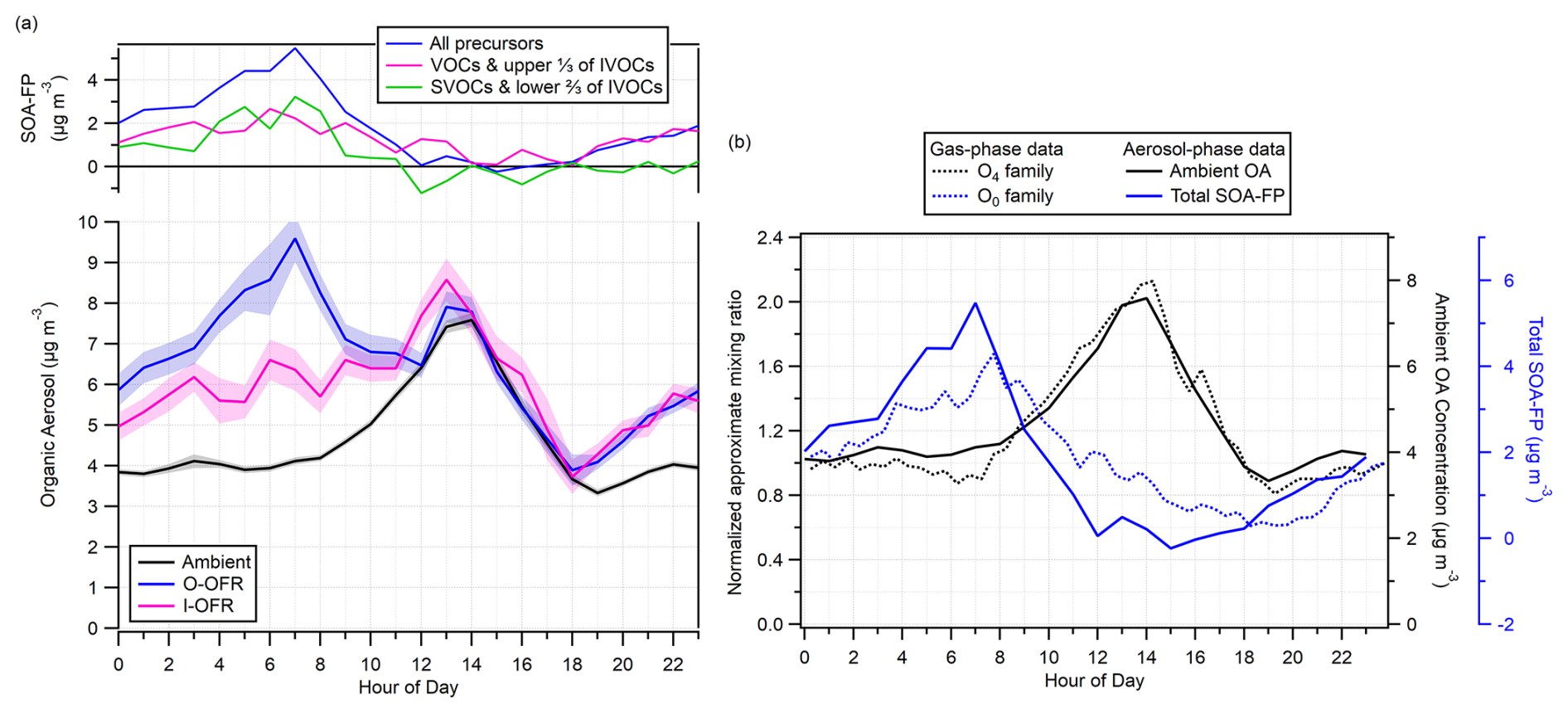
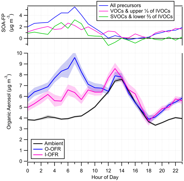
Figure 6 (a) Diurnal cycles (1 h time resolution) of OA through each sampling pathway: ambient air, O-OFR and I-OFR (bottom). Shaded regions indicate ±1 standard error. (a) SOA-FP from all precursors (O-OFR minus ambient), precursors in the VOC and upper $\mathrm{1}/\mathrm{3}$ of IVOC volatility range (I-OFR minus ambient), and SOA-FP from all lower-volatility precursors (O-OFR minus the I-OFR) (top). (b) A comparison of the ambient OA and total SOA-FP from panel (a) with families of gas-phase species based on the number of oxygens.

The campaign-averaged diurnal cycles of OA through the different sampling pathways are shown in Fig. 6a. Ambient air had an OA concentration of 4 µg m⁻³ during the morning and night, with a peak at 7.5 µg m⁻³ in the afternoon. Ambient OA had a general trend of increasing with increasing temperature (Fig. S9); when only midday (11:00–16:00 PDT) data were analyzed, the temperature dependence was flat or slightly decreasing with increasing temperature. The O-OFR, which ingested all precursors, formed an average of 2.1 µg m⁻³ of SOA on top of ambient; this ranged from zero in the afternoons to 5.5 µg m⁻³ in the mornings. The I-OFR, which only ingested higher-volatility precursors, formed an average of 1.3 µg m⁻³, with a similar diurnal pattern.

The amount of SOA formed on top of ambient (SOA-FP) is plotted on the top panel of Fig. 6a. The SOA-FP measured in the I-OFR represents SOA formed only by VOCs and the upper third of IVOCs, and the SOA-FP measured in the O-OFR represents SOA formed by all precursors. The difference between the two represents SOA formed by lower-volatility precursors. These are the first measurements we know of that quantify SOA-FP from ambient air that has been experimentally split into two volatility ranges. The SOA-FP data are noisiest from 12:00–18:00 PDT, when the OFRs have collapsed onto the ambient measurement, because there is little to no SOA formation above ambient during this period. A nightly average (22:00–08:00 PDT) of SOA-FP for both OFRs is shown in Fig. S10, along with the same data normalized to ΔCO. The SOA-FP was fairly constant over the campaign and did not vary between weekdays and weekends, as shown in Fig. S11. We also explored the dependence of SOA-FP on ambient temperature (Fig. S12). We did not find a clear trend, except that in the early morning (06:00–08:00 PDT) the I-OFR SOA-FP seems to positively correlate with temperature.

In Fig. 6a, the growth of SOA-FP due to lower-volatility precursors starts to be significant around midnight and peaks at 07:00 PDT in the morning. When the photochemical age is highest (afternoon), the measured SOA-FP drops to zero. Since the contribution of lower-volatility precursors is highest when the photochemical age is lowest, this suggests that the dominant source of lower-volatility precursors is primary emission, rather than multigenerational oxidation. One exception is products of NO₃ radical oxidation of monoterpenes, which do accumulate at night. Figure 11a shows the relatively small contribution to SOA-FP from these intermediate species. The lack of measurable SOA-FP in the afternoon also indicates that oxidation has exhausted SOA-FP, and there is no further SOA to be formed by aging multigenerationally across days.

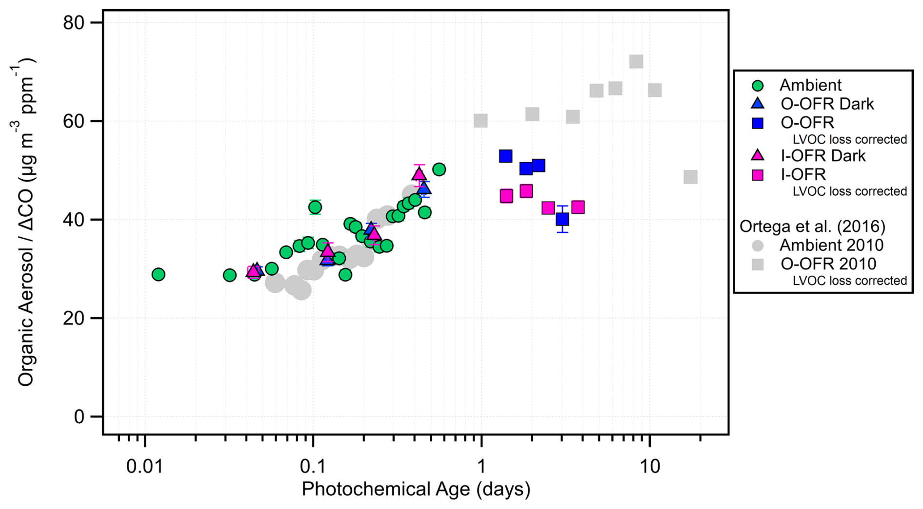
Figure 7 Quantiles of OA, normalized by ΔCO, plotted as a function of total photochemical age (the sum of ambient age and the additional aging in the OFR). All data points have standard errors as the vertical and horizontal error bars; most error bars are smaller than the drawn markers. For the OFRs, “dark” periods correspond to measurements with the lamps off. Results are shown with the LVOC loss correction described in Sect. 3.3. Gray points are data from 2010 for comparison. During the 2010 campaign lamp stepping was used in the OFR to probe higher photochemical ages, and in this campaign the photochemical age was targeted to be constant at ∼ 2 d.

Further evidence to support the lower-volatility precursors being emitted rather than formed is shown in Fig. 7b. In their analysis of the Vocus data from this campaign Blauth et al. (2026) grouped the gas-phase species according to the number of oxygens. The least and most oxygenated O_x families are plotted in Fig. 6b, with concentrations normalized to be 1 at midnight. The O₄ family peaks in the afternoon, and its diurnal cycle is nearly identical to the ambient SOA trace when overlaid. The O₄ family anti-correlates with the total SOA-FP measured in the O-OFR. Despite the presence of these highly oxygenated VOCs in the afternoon there is no measured SOA-FP. Again, this strongly suggests that the dominant source of lower-volatility precursors is primary emission, rather than multigenerational oxidation. The O₀ family peaks in the morning, similar to the total SOA-FP, and is anti-correlated with ambient SOA. This is consistent with the analysis we present in Sect. 3.8, where we find that non-oxygenated species correlate best with total SOA-FP.

One limitation of this technique is that we are unable to experimentally determine if precursor identities changed between morning (when substantial SOA-FP is measured in the OFRs) and afternoon (when SOA-FP is realized via photochemistry in ambient air). In Sect. 3.9.4 we explore this topic in more detail via modeling, using the data in Fig. 13c. During late night into morning, the O-OFR forms a similar amount of total OA to the afternoon peak ambient OA (∼ 7.5 µg m⁻³), indicating consistency in the total magnitude of OA and little additional SOA-FP from further oxidation during afternoon. A similar result was observed at a nearby site by Ortega et al. (2016) during the CalNex-2010 experiment.

To understand the effect of the diurnal cycle of the planetary boundary layer (PBL) height on these measurements, Fig. S13 compares the surface concentrations of OA from Fig. 6a with estimated column-integrated concentrations. The column-integrated concentrations show more moderate variations at night and the early morning, due to the effect of the changing PBL height. The column-integrated SOA-FP still collapses onto the ambient data at noon.

A comparison of ambient data from 2010 and 2022 is made in Fig. 7. Quantiles of OA, normalized to ΔCO, are plotted as a function of photochemical age. Normalizing to ΔCO corrects for dilution of emissions. We used a background CO value of 100 ppb as determined by Schulze et al. (2025) from correlations of CO with reactive aromatic species and NO_y. Ambient data appear unchanged between 2010 and 2022 in both the amount of SOA formation and the approximate photochemical age range. Under a day of aging, it is expected that SOA formation is positively correlated with increasing age (Hayes et al., 2015), which is true for the ambient data from both years.

Figure 7 also shows a comparison of OFR data from 2010 and 2022. Each OFR was plotted as a function of total photochemical age, which was the sum of ambient age and the additional aging in the OFR. The OFR data from 2022 span a narrower photochemical age range than 2010 by experimental design. Rather than step through various photochemical ages, as was done in 2010, both the OFRs for this campaign were tuned to a constant ∼ 2 d of aging in order to capture higher-time-resolution data near the expected peak production exposures. In this photochemical age range (1–10 d), we do not expect SOA formation to be dependent on age, based on previous campaigns (Ortega et al., 2016; Palm et al., 2016). The plateau of SOA-FP $/$ ΔCO as photochemical age increases was measured in both 2010 and 2022 and indicates that SOA precursors are being exhausted by the photochemical aging level reached by the OFRs. In 2010, the OFR did not have an inlet and should therefore be compared to the O-OFR from 2022. Other than the “dark” periods, where the OFRs were measured with the lamps off, all OFR data in Fig. 7 are shown with the low-volatility organic compound (LVOC) loss correction described in Sect. 3.3. The correction shifts the data higher by accounting for non-atmospherically relevant losses of LVOCs occurring in the OFR.

Total OA (including SOA-FP) has decreased ∼ 10 µg m⁻³ ppm⁻¹ since 2022. Precursor concentrations directly impact SOA-FP. While hydrocarbons have decreased in concentration since 2010, oxygenated VOCs have remained similar or increased (Jensen et al., 2024). Analysis from Jensen et al. (2024) shows that ambient photochemistry in LA has become faster in the last decade. The average OH exposure during this campaign was ∼ 68 % higher during midday than in 2010. Higher OH exposure leads to faster oxidation. This consumes SOA precursors during transport to the measurement site in Pasadena. Combined with a decrease in precursors since 2010, it helps explain similar amounts of SOA but decreased SOA-FP.

3.3 Quality assurance and data corrections

The automated sampling system was evaluated in multiple ways to ensure high data quality. The system had several rotameters installed on excess flow lines so that, daily, a visual flow check could ensure co-sampling of pathways never occurred (a photo of the rotameter system is shown in Fig. S14). Additionally, CO₂ was monitored in the O-OFR, inside the penthouse and outside, which allowed for an analysis of potential leaks. Due to occupancy by the researchers, CO₂ inside the penthouse was consistently at least double the outdoor value. After extended periods of being unoccupied, the penthouse CO₂ equilibrated with outdoor concentrations, allowing a check of the consistency of all three sensors. We confirmed that the O-OFR CO₂ measurement matched the outdoor value and was not tracking the indoor values, indicating that the system was sealed from indoor air influence. The inlet of the I-OFR was co-located with the O-OFR and therefore also protected from indoor air.

To determine if a correction for aerosol transmission was necessary, both OFRs were run with the lamps off for 20 min every 6 h. Figure S15 shows the concentration of SO₄ measured in the OFRs during lights-off periods against the amount measured in ambient air. Sulfate aerosol was used as a proxy for all aerosols to determine wall losses as it is nonvolatile and typically internally mixed with OA. We found that the O-OFR did not need a correction for aerosol transmission compared to the ambient measurements, while the I-OFR needed a correction of +16 % (Fig. S15). Since the O-OFR did not require a correction, and the two OFRs are made of the same material, it is highly likely that aerosol losses were occurring in the inlet sampling path as opposed to the OFR itself. Losses could have occurred in the cPFA tubing, the non-conductive Teflon fittings, the three-way non-conductive Teflon solenoid valves or the general turbulence caused by curves in the tubing. The correction factor was only applied to ambient aerosols entering the OFR and not to aerosols generated inside the OFR. This was achieved using Eq. (1) below:

$$\begin{array}{}\text{(1)}& {\mathrm{OA}}_{\text{I-OFR corrected}}={\mathrm{OA}}_{\text{I-OFR}}+\left({\mathrm{OA}}_{\mathrm{Ambient}}\right)\left(\mathrm{0.161}\right),\end{array}$$

where OA_{I-OFR corrected} is the corrected value for OA in the I-OFR, OA_I-OFR is the original uncorrected value, and OA_Ambient is the interpolated ambient value for OA for the given time period.

To determine if a correction was necessary for non-atmospherically relevant losses of condensable gases (low-volatility organic compounds, LVOCs) in the OFRs, we used the methods of Palm et al. (2016). The dominant LVOC loss pathway outdoors is condensation onto aerosols; however, inside the OFRs other LVOC fates include (i) condensation onto the walls of the OFR; (ii) continued oxidation leading to fragmentation; and (iii) exiting the OFR before having time to condense to particles, thus depositing on tubing walls. A previously published model (Palm et al., 2016) was used to calculate the estimated fraction of LVOC fates in each OFR. The LVOC fate model was initially developed to correct OFR data in a pine forest. The proportion of LVOCs condensing onto aerosols has a strong dependence on the aerosol condensational sink; at ∼ 1 d of photochemical aging in a pine forest, higher (lower) condensational sinks led to ∼ 60 % (∼ 20 %) condensation onto aerosols (Palm et al., 2016). To estimate the condensational sink in the OFR model, we average the input and output condensational sinks (calculated from the SMPS data). For ∼ 1 d of photochemical aging in LA in 2010, 80 % of LVOCs were condensing onto aerosols (Ortega et al., 2016).

The average fraction of LVOCs condensing onto aerosols was 43 % in the O-OFR and 38 % in the I-OFR in this study. Figure S16a shows the time series of LVOC fractional fates; each non-atmospherically relevant pathway consumed ∼ 20 % of LVOCs on average. Since this correction should only be applied to aerosols generated in the OFRs and not to ambient aerosols, the correction was applied using Eq. (2) below:

$$\begin{array}{}\text{(2)}& {\mathrm{OA}}_{\mathrm{OFR}\mathrm{corrected}}={\displaystyle \frac{({\mathrm{OA}}_{\mathrm{OFR}}-{\mathrm{OA}}_{\mathrm{Ambient}})}{F_{\mathrm{cond}}}}+{\mathrm{OA}}_{\mathrm{Ambient}},\end{array}$$

where OA_{OFR corrected} is the corrected value for OA in the OFR, OA_OFR is the original uncorrected value, OA_Ambient is the interpolated ambient value for OA for the given time period, and F_cond is the calculated fraction of LVOCs that have condensed onto aerosols. This correction was applied after correcting for aerosol transmission.

The variability in condensation onto aerosols was better explained by variability in condensational sink rather than OH exposure (Fig. S16b, c). The measured condensational sink for each pathway (Fig. S17) followed the same average diurnal cycle as the OA shown in Fig. 6a. Ambient air had a background condensational sink of 0.004 s⁻¹ and peaked at 0.007 s⁻¹ in the afternoon.

If the OFRs are run at high lamp power, it is possible that the temperature enhancement inside the OFR compared to outside the OFR can cause evaporation of OA (Pan et al., 2024). When operated at the average campaign lamp power settings, the measured temperature enhancement inside our OFRs was 1–2 °C. Pan et al. (2024) estimate the evaporation rate of OA in the OFR to be 1 × 10⁻⁴–2.5 × 10⁻⁴ s⁻¹ °C⁻¹. Using this range, we estimate an average of 5 % (range 2 %–9 %) of the ambient OA could have evaporated inside the OFR during our experiments. We did not correct the data for potential OA evaporation as the effect would have been small compared to the inherent uncertainties already in the experiments.

For several analyses results were normalized to background-corrected carbon monoxide (ΔCO). Normalizing to ΔCO removes some of the real variability in dilution and air mass transport. To determine ΔCO, measured CO was subtracted by a background average of 100 ppb as calculated in Schulze et al. (2025).

3.4 Photochemical age in the OFRs

OA generation in OFRs has been shown to have a non-linear dependence on OH exposure: for up to 1 d of aging OA generation is positively correlated with OH exposure, at 1–10 d of aging OA generation plateaus and does not have a dependence on OH exposure, and at ages higher than 10 d OA may begin to be destroyed as OH exposure increases (Ortega et al., 2016). For this reason both OFRs were tuned to ∼ 2 d of equivalent exposure. The actual exposures of both OFRs were slightly different, due to the difficulty of precisely tuning the exposure in the field. Figure S18 shows no correlation between OA and OH exposure for either OFR. Therefore, no correction for differing photochemical ages was necessary to quantitatively compare OA between the two OFRs.

The OH exposure was calculated for each OFR according to the toluene decay method described in Sect. 2.4. Assuming a daily average concentration of OH of 1.5 × 10⁶ molec. cm⁻³, the O-OFR contributed an additional 1.8 ± 0.6 (1σ) days of aging on top of ambient age, and the I-OFR contributed an additional 2.6 ± 1.2 (1σ) days of aging on top of ambient age. The midday ambient photochemical age was determined by Jensen et al. (2024) to be ∼ 0.5 d, while ambient photochemical ages at other times were lower. Figure S19 shows an example toluene time series demonstrating decays during OFR measurements, as well as the corresponding photochemical age.

In Jensen et al. (2024) the reported photochemical age for the O-OFR (∼ 1 d) was estimated via hydrocarbon ratios of C₈ and C₉ aromatics compared to benzene, following previously developed methods (Hayes et al., 2013). This estimation technique is optimized for outdoor air, where fast-reacting C₈ and C₉ aromatics decay a measurable amount during the day compared to nighttime concentrations. However, in the OFRs C₈ and C₉ aromatics decayed completely, making this technique susceptible to underestimation of OH exposure. We believe that using toluene, which on average decayed 71 % and 88 % in the O-OFR and I-OFR respectively, provides a more accurate estimation of OH exposure for the OFRs.

A comparison of the OH exposure calculated using real-time ambient toluene decays in the OFR and the OFR estimation equation from Li et al. (2015) is shown in Fig. S20. We found that the estimation equation results were correlated with the toluene decay results but overestimated OH exposure by a factor of ∼ 2, which is typical of similar comparisons in past experiments (Palm et al., 2016).

3.5 Measurement–model comparisons

The modeling results for total OA and SOA-FP are shown in Fig. 8, overlaid on the measurement data from Fig. 6a. The diurnal cycle of ambient OA for CRACMM was directly output from CMAQ. The overall magnitude and diurnal variation is very similar to the observations, with the exception that the modeled ambient OA peaks about 2 h earlier. Ambient OA from the Caltech model had a similar diurnal cycle to observations but on average was ∼ 1.5 µg m⁻³ lower.

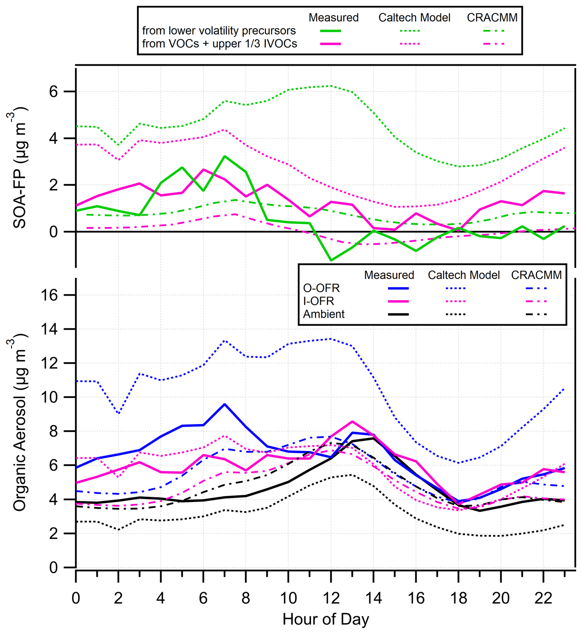
Figure 8 Comparison (as a diurnal average) of measured results to the Caltech model and CRACMM mechanism (ambient results for CRACMM are CMAQ output). Bottom: OA vs. diurnal hour for ambient air and the outputs of both OFRs. Top: SOA-FP for the two precursor volatility ranges. The higher volatility range is calculated as the difference in total OA between the I-OFR and ambient air. The lower volatility range is calculated as the difference in total OA between the O-OFR and the I-OFR.

As described in Sect. 2.6, both models were adapted to simulate the photochemical aging of the O-OFR and I-OFR. Modeled total OA for the OFRs is compared to measurements in the bottom of Fig. 8. The CRACMM O-OFR simulation underpredicted total OA by 1.4 µg m⁻³ on average in the morning (00:00–12:00 PDT). The Caltech model overestimated the total OA in the O-OFR by 4.5 µg m⁻³ on average in the morning (00:00–12:00 PDT). The total OA in the I-OFR appears to match well between the Caltech model and the observations, but this is because the underestimation of the ambient OA is compensating for the overestimation in I-OFR SOA-FP.

The top panel of Fig. 8 shows model–measurement comparisons for SOA-FP according to the volatility split of precursors. The SOA-FP for the higher volatility range was calculated as the difference in total OA between the I-OFR and ambient air, and the SOA-FP for the lower volatility range was calculated as the difference in total OA between the O-OFR and I-OFR. CRACMM simulations for SOA-FP were underestimated compared to the observations but followed a similar diurnal profile. The Caltech box model overestimated the SOA-FP for both volatility ranges at all hours. The most noticeable departure from the observed SOA-FP was in the afternoon, when measurements had collapsed to near zero, but the Caltech box model was still producing 6 µg m⁻³ from lower-volatility precursors.

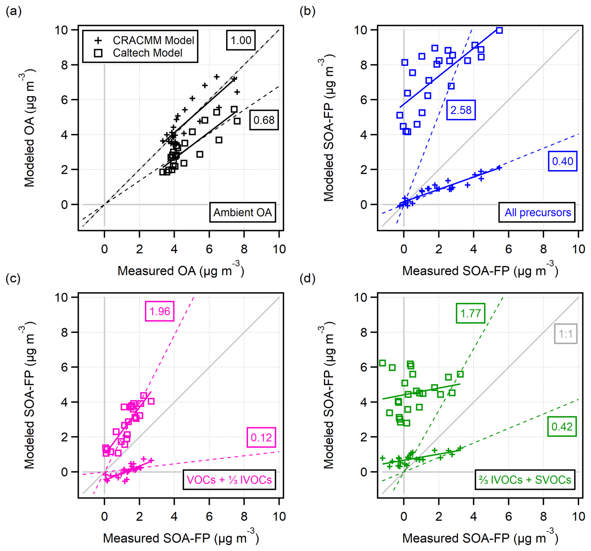
Figure 9 (a) Modeled ambient OA from the CMAQ and Caltech models vs. measured ambient OA. Each data point represents an average diurnal hour. (b–d) Modeled SOA-FP from different precursor volatility groups vs. measured SOA-FP. For all plots, the data were linearly fit with the intercept fixed at zero and free. Slopes are shown for the fits with the intercept fixed at zero. See Table S4 for slopes of the fits without fixed intercept.

Scatterplots in Fig. 9 are used to quantify how well the models agree with the measurements. Figure 9a compares ambient OA: CRACMM matched the measurements very well, while the Caltech model underestimated OA by 32 %. Figure 9b–d show the model–measurement comparison of SOA-FP from all precursors and precursors split by volatility. The Caltech model overestimated the SOA-FP from all precursors by a factor of 2.6, and CRACMM underestimated SOA-FP from all precursors by a similar factor.

There are many possible reasons for the model–measurement discrepancies discussed above, including uncertainties in emissions, gas-phase oxidation chemistry, volatility distributions or gas–particle partitioning yields. To test if uncertainties in emissions affect the amount of SOA-FP, CRACMM was also run with the unconstrained CMAQ output as input. This resulted in enhanced SOA-FP in the O-OFR and I-OFR from 05:00–12:00 PDT, bringing the model into slightly better agreement, but otherwise looked very similar to the constrained results (Fig. S21). Unfortunately, we do not currently have a way to deconvolve the possible effects of the other listed factors from one another.

3.6 Breakdown of total SOA potential by volatility and source

The O-OFR ingested all precursors, and the I-OFR ingested only precursors with a high enough volatility to transmit through the inlet. This allows us to report the first ambient measurements of SOA-FP with an experimental volatility split. Figure 10 shows the SOA-FP results from Fig. 8 stacked to compare the measured and modeled total SOA-FP at different times of day. Compared to the observations, CRACMM underpredicts SOA-FP, and the Caltech model overpredicts SOA-FP. As discussed earlier, in the afternoon, measured SOA-FP collapses to near zero. CRACMM captures this trend with the exception of some extra SOA-FP from lower-volatility precursors. The Caltech model does not capture this trend.

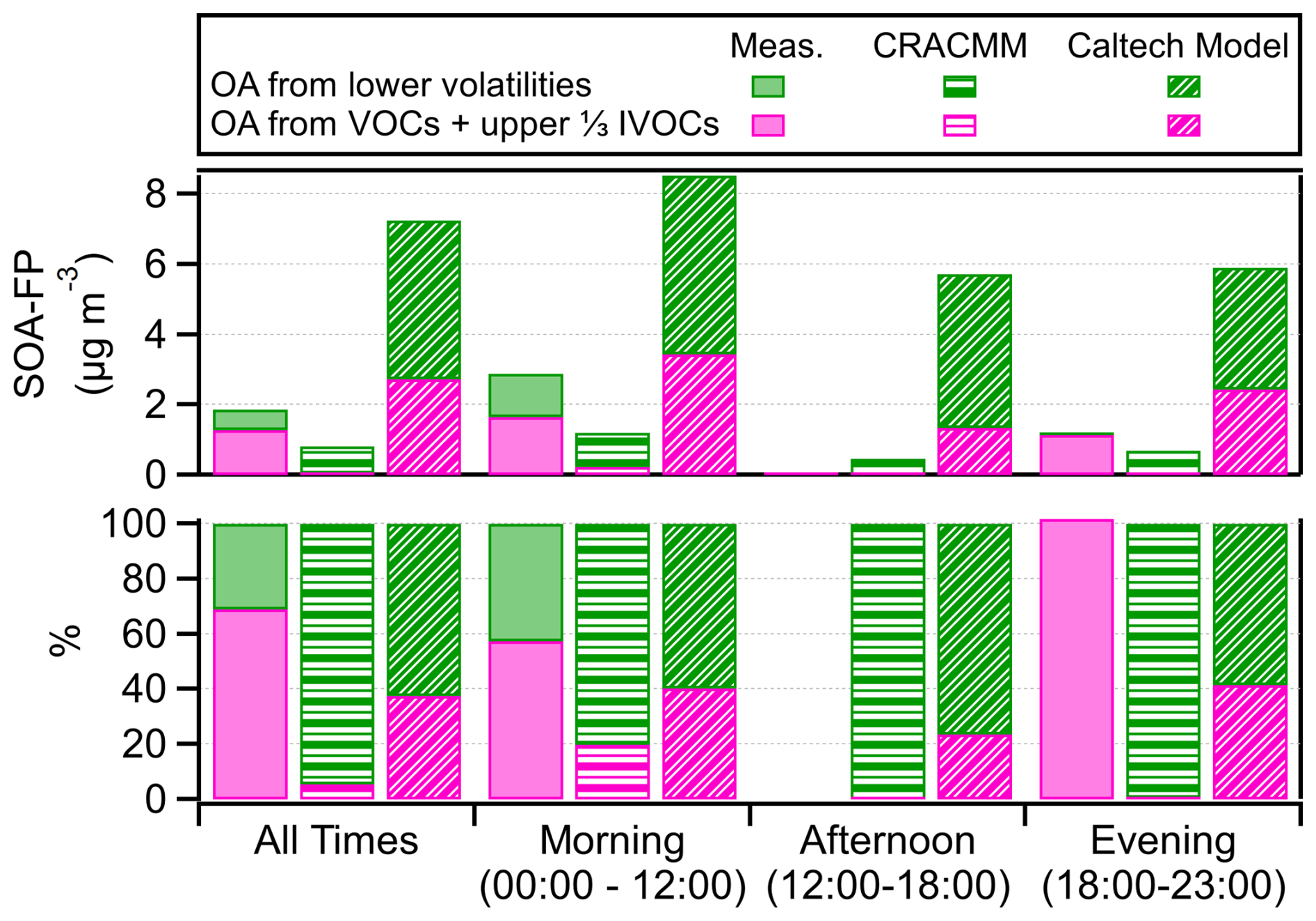
Figure 10 Measurement–model comparison of SOA-FP split by precursor volatility range. The pink bars indicate SOA that was formed by precursors transmitted through the inlet of the I-OFR (VOCs and upper $\mathrm{1}/\mathrm{3}$ IVOCs). The green bars indicate SOA that was formed by all other precursors (SVOCs and lower $\mathrm{2}/\mathrm{3}$ IVOCs). The diurnal cycle data from Fig. 8 were averaged over the specified time periods to calculate the values shown. The top panel shows the absolute magnitudes, while the bottom panel shows the same data as percentages. The percent afternoon measurement bar is omitted because the absolute SOA-FP for this period was near zero.

The bottom panel of Fig. 10 shows the same data as percentages. Our measurements indicate that 69 % of the average daily SOA-FP is attributed to precursors in the VOC and the upper $\mathrm{1}/\mathrm{3}$ IVOC range. This estimate varies from 57 %–100 % depending on the averaged time period, as shown in Fig. 10. Importantly, this result refers to the SOA-FP present in the gas phase in LA and does not inform the precursor volatility breakdown of the ∼ 4 µg m⁻³ ambient OA background seen at all hours.

Over the whole diurnal, both models underestimated the fractional contribution to SOA-FP of high-volatility precursors significantly. The closest model–measurement agreement is seen for the morning time period, which is when SOA-FP is highest. The afternoon measured SOA-FP percent is omitted because the SOA-FP was near zero. In the evening we measure 100 % of the SOA-FP as from higher-volatility precursors, but the CRACMM attributes almost all of it to lower-volatility precursors, and the Caltech model remains closer to a 50 : 50 split of SOA-FP from higher- vs. lower-volatility precursors.

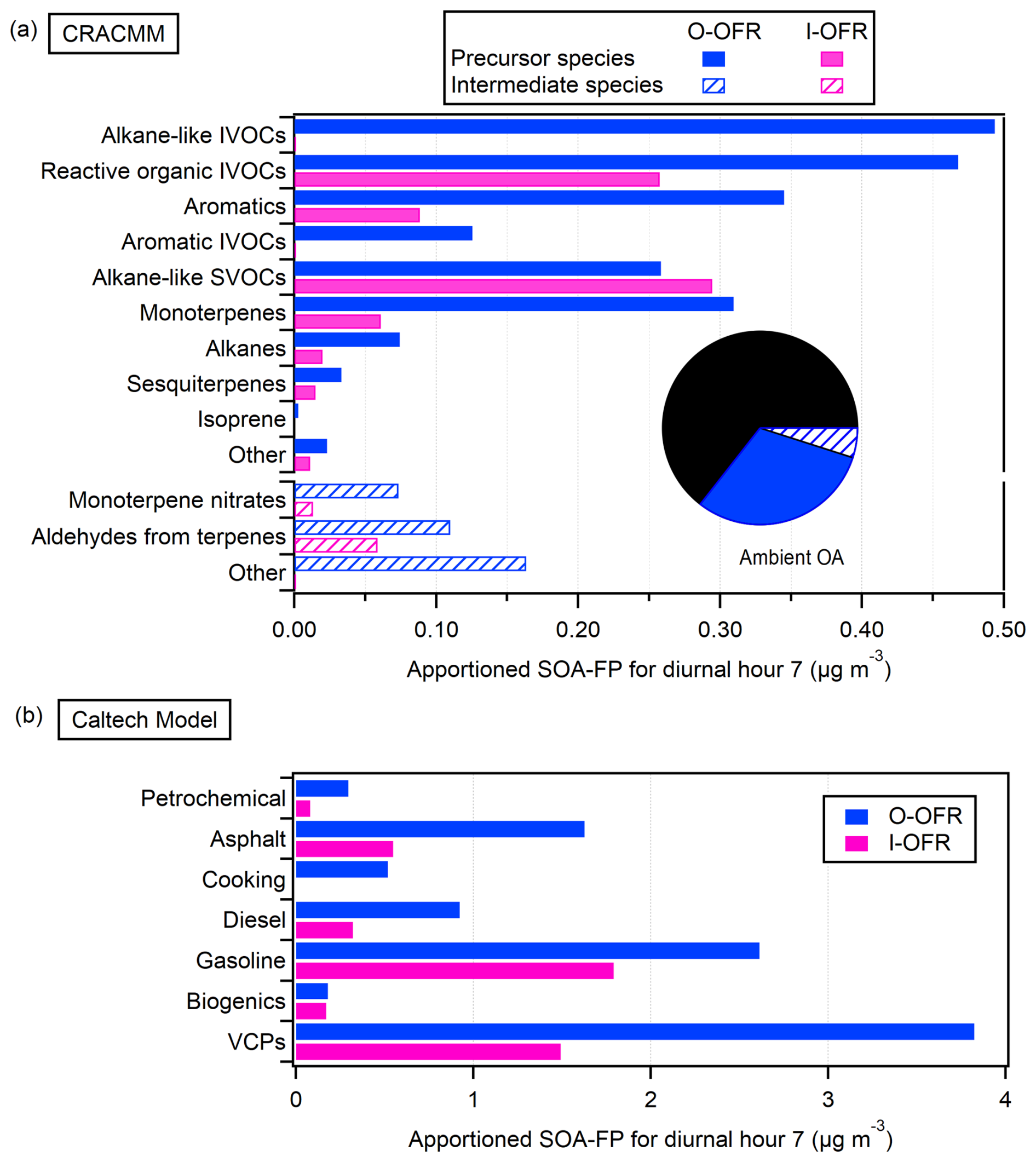
Figure 11 SOA-FP from 07:00 PDT in the morning for each OFR apportioned to species categories or sources, for (a) CRACMM and (b) the Caltech model. Contributions to ambient SOA (that have already formed when the air enters the OFRs) have been subtracted off. The inset pie chart in panel (a) is equal to the total OA modeled for the O-OFR for 07:00 PDT. The Caltech model results can be further split by volatility, which is shown in Fig. S22.

To investigate specific contributions to SOA-FP, we ran a source apportioning case study on the OFR modeling results for 07:00 PDT in the morning, when measured SOA-FP was highest. The Caltech model is built on source-based inventory estimates, and the amount of SOA-FP formed in each OFR (with contributions to ambient subtracted off) per source is shown in Fig. 11b. VCPs accounted for ∼ 40 % of the total SOA-FP, followed by gasoline and asphalt. Biogenics (isoprene and monoterpenes) made very little additional SOA on top of ambient. The Caltech results can also be split according to volatility, which is shown in Fig. S22.

Source apportioning in CRACMM was more involved, as CRACMM has over 200 species participating in a complex set of chemical reactions. To apportion the SOA-FP for 07:00 PDT, we initialized each species to zero, one at a time. The difference between the total OA in the original case and the total OA with one species initialized to zero was considered to be the SOA-FP attributed to that species. Importantly, we constrained the partitioning OA concentration and kinetics to match the original case to remove partitioning effects. If CRACMM was an entirely linear model system, the sum of each apportioned SOA-FP per species would be equal to the total OA modeled for the O-OFR. This was not true, indicating some intermediate species contribute to SOA in non-linear ways. To obtain meaningful results, we separated all the species into three categories: (i) species in the aerosol phase, (ii) species in the gas phase that were not formed by any reactions (precursors) and (iii) species in the gas phase that were formed by at least one reaction (intermediates).

The inset pie chart in Fig. 11a is equal to the total OA modeled for the O-OFR. The wedges represent OA from aerosol species and SOA from precursors, and the calculated leftover SOA is attributed to intermediates. Figure 11a shows the CRACMM apportioning results according to grouped species. The largest contributors to total SOA-FP were alkane-like IVOCs and reactive organic IVOCs, the latter of which was denuded by the inlet of the I-OFR.

3.7 Model sensitivity tests

Overestimation of SOA production in a chemical mechanism can occur due to absorptive partitioning feedback, as semi-volatile SOA is highly sensitive to the amount of aerosol present (Bian and Bowman, 2005). To test how sensitive the models were to the amount of preexisting OA, the total OA from 07:00 PDT (where measured SOA-FP was highest) was input into a separate model experiment. All chemistry was turned off, and the OA was allowed to repartition according to a prescribed seed concentration, with a constant condensational sink of 1 s⁻¹. This calculation was done for both models for all three sampling pathways. By exposing the OA to lower prescribed seed OA concentrations we quantify the amount of expected OA evaporation, and by exposing the OA to higher prescribed seed OA concentrations we quantify the amount of expected OA condensation. This gives an indication of how sensitive each model is to changes in the amount of partitioning aerosol.

Results in Fig. S23 show a weak sensitivity to evaporation and condensation. When the O-OFR output was exposed to an order of magnitude less seed OA, 9 % of the OA from CRACMM and 29 % of the OA from the box model evaporated. When exposed to an order of magnitude more seed OA, an additional 3 % of the original OA from CRACMM and 16 % of the original OA from the box model condensed. The results also indicate that there is a significant fraction of OA in CRACMM that is effectively non-volatile, as about half the OA did not evaporate even at very low (0.01 µg m⁻³) seed concentrations. Unlike CRACMM, the box model did not have much non-volatile OA; at very low (0.01 µg m⁻³) seed concentrations the OA for all model runs had evaporated to less than 0.5 µg m⁻³.

SOA formation also depends on the photochemical age reached inside the OFR. To quantify how sensitive the model results were to age, we used as input the predicted ambient concentrations for 07:00 PDT, and both the O-OFR and the I-OFR models were simulated up to an exposure of 5 d of aging (on top of ambient). The results in Fig. S24 show an exponential rise in SOA formation from 0–1.5 d, and then results begin to plateau. SOA formation in both models had little dependence on age at the experimental photochemical ages for both OFRs. Also included is a simulation from the Hayes et al. (2015) SIMPLE model for urban SOA formation. The SIMPLE model uses two parameters, a single concentration of a precursor VOC (with an SOA yield of 100 %) and a single rate coefficient, to model SOA formation as a function of photochemical age. These parameters have previously been fit to the CalNext-2010 measurements in LA, with ΔVOC $/$ ΔCO = 80 µg m⁻³ ppmv⁻¹ and a kOH = 12 × 10¹² cm³ molec.⁻¹ s⁻¹, and were similar to results in Mexico City and other locations (Hodzic and Jimenez, 2011; Nault et al., 2021). We used these fit parameters and a measured ΔCO for 07:00 PDT of 0.156 ppmV to run the model. SIMPLE formed twice as much SOA as CRACMM but had a similar dependence on photochemical age. This confirms the results of Fig. 7, showing reduced SOA-FP per unit CO in LA since 2010. A value of ΔVOC $/$ ΔCO = 37 µg m⁻³ ppmv⁻¹ would match the observations.

To understand the dependence of simulated OA on the inlet transmission curve, we ran I-OFR simulations with more and less denuding than our estimate from Fig. 3. The results for CRACMM in Fig. S25 appear very similar; with the inlet denuding an order of magnitude more or less volatile precursors, the total OA was only ±0.1 µg m⁻³ different on average. For the Caltech model (Fig. S26), also a small ±0.5 µg m⁻³ average difference is observed. This indicates that uncertainties in the transmission curve are not a major influence on the model results.

3.8 Precursor correlation with SOA formation potential

We investigate the possible sources of SOA precursors by correlating the SOA-FP measured in each OFR with VOC time series (as tracers of different sources). Pearson R² values between VOCs and SOA-FP from both OFRs are shown in Fig. S27. Figure 12a shows a representative subset of the time series where SOA-FP is overlapped with the top three most correlated VOCs. For the 2010 CalNex experiment in LA Ortega et al. (2016) reported that 1,3,5-trimethylbenzene was very strongly correlated in time with SOA-FP (R² of 0.67), although the amount of SOA that could be formed from this precursor was much lower than the total SOA-FP measured. By contrast the correlation of biogenic species with the measured SOA-FP was very low. We compare our results to those from 2010 in Fig. S28. We found that 1,3,5-trimethylbenzene has decreased in correlation with SOA-FP (R² of 0.36). We speculate that since the relative importance of traffic and mobile sources for SOA formation decreased from 50 % in 2010 to 25 % in 2022 (Schulze et al., 2025), and 1,3,5-trimethylbenzene is an anthropogenic emission (Wyche et al., 2009) associated with gasoline, the correlation would decrease as other sources become important. Isoprene remains uncorrelated with measured SOA-FP. Monoterpenes, which were unspeciated in our Vocus measurements, had an R² value of 0.19. In 2010, the R² value for α-pinene was 0.001.

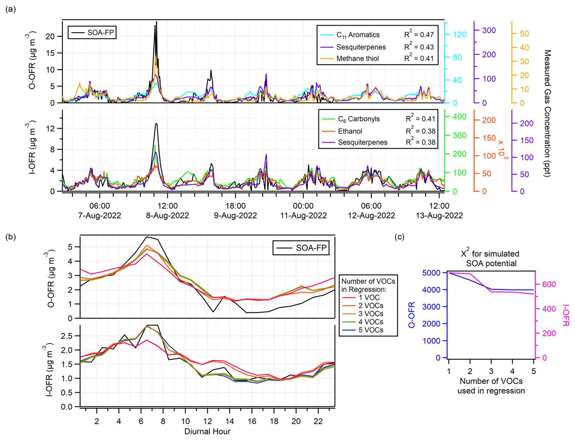
Figure 12 (a) A time series of SOA-FP in each OFR, overlaid with the top three most correlated gas-phase precursors. (b) A diurnal of SOA-FP in each OFR, overlaid with the simulated SOA-FPs (diurnally averaged results of the multiple linear regressions). (c) The sum of squared residuals for each regression as a function of the number of VOCs used.

The top five VOCs most correlated with SOA-FP were used in a multiple linear regression to create a simulated SOA-FP time series, which was then compared to the experimental results. The multiple linear regression equation is

$$\begin{array}{}\text{(3)}& \begin{array}{rl}{\text{SOA-FP}}_{\mathrm{simulated}}=& a\times \mathrm{VOC}a+b\times \mathrm{VOC}b+c\times \mathrm{VOC}c\\ & +\mathrm{\dots },\end{array}\end{array}$$

where SOA-FP_simulated is the result of the linear regression, a is the regression coefficient for VOCa, and so on. Some precursors in the top 10 most correlated list for each OFR were highly correlated with each other (R² > 0.70) and were replaced with the next most-correlated species. Figure S29 shows a matrix of VOC–VOC correlations. While some functionally similar species like C_8–12 alkyl aromatics were highly correlated with each other, other chemically similar species like C_6–9 carbonyls were not. For the O-OFR, C₁₁ aromatics, sesquiterpenes, methanethiol, styrene and C₆ carbonyls were used in the regression (with an R² range of 0.31–0.47). For the I-OFR, C₆ carbonyls, ethanol, sesquiterpenes, C₁₁ aromatics and styrene were used in the regression (with an R² range of 0.30–0.41). A list of fitting coefficients is shown in Table S5. Interestingly, some of the fit coefficients (e.g., for ethanol) were zero. This indicates that those VOCs, while correlated with SOA-FP and not well correlated with the other VOCs in the regression, were not needed to explain the variance of the SOA-FP. The simulated SOA-FP is shown as an averaged diurnal in Fig. 12b and has relatively good agreement with the OFR data. The difference between having one VOC in the regression vs. five VOCs in the regression was minimal.

The top five most-correlated VOCs can explain the variance of the SOA-FP well, but they cannot explain the actual mass attributed to them by the regression. We calculated the maximum amount of SOA that could form from the precursors using SOA yields from the literature and include those estimates in Table S5. All the estimates are significantly lower than the attributed SOA mass. These precursors are therefore understood to be tracers of SOA-FP and represent the SOA-FP mass from all compounds that correlate with them. For example, carbonyls have been shown to be associated with cooking emissions (Coggon et al., 2024a) and C_10–11 aromatics with asphalt emissions (Khare et al., 2020).

3.9 Discussion of results on the importance of terpenes for SOA-FP

We compare results about the contribution of biogenic and anthropogenic terpenes to ambient SOA in summer in Los Angeles in Fig. 13a. Results from the CalNex-2010 study concluded that biogenic monoterpenes were responsible for 1 %–4 % of ambient SOA through both modeling and gas chromatography mass spectrometry tracer analysis (Hayes et al., 2015; Ma et al., 2017). Only 29 % of the ambient SOA formed from urban emissions was comprised of modern carbon, much of which was attributed to VCPs of modern carbon origin and cooking emissions (Zotter et al., 2014). SOA formed regionally and advected into the LA Basin as SOA (not as SOA-FP) did include a larger biogenic fraction from, for example, the California Central Valley (Hayes et al., 2013, 2015; Heo et al., 2015; Zotter et al., 2014). Ambient SOA-FP during CalNex-2010 had a similar diurnal cycle as in this study and was strongly correlated with short-lived aromatics such as trimethylbenzene; it had low correlation with biogenics such as isoprene, limonene and α-pinene (Ortega et al., 2016). An analysis from multiple large megacities worldwide concluded that aromatic reactivity was the best predictor of the amount of SOA formed (Nault et al., 2021). Those studies were conducted in 2000–2016, and anthropogenic emissions have been significantly reduced since (Jensen et al., 2024; Schafer et al., 2025). Schulze et al. (2025), with the Caltech model used as starting point for our study, estimated that 14 % of ambient SOA is from biogenic terpenes for LA in 2022, and 7 % is from anthropogenic terpenes (from VCPs), almost double their results for 2010. Biogenic and anthropogenic terpene sources being both important in urban areas is supported by recent studies (Katz et al., 2025; Tasnia et al., 2026).

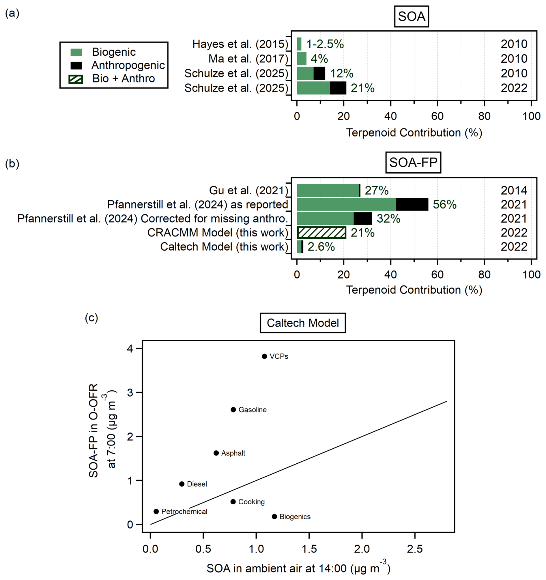
Figure 13 (a) A bar plot summarizing the literature on terpene contributions to ambient SOA in Los Angeles, as percentages. Results are split between biogenic and anthropogenic sources. The years of the studies are indicated on the right. (b) A summary of estimates of terpene contribution to total SOA-FP in LA. The Pfannerstill et al. (2024) “as reported” bar has an error of ±33 %. The anthropogenic contribution shown here is an average of the possible percentages they report. The CRACMM bar for this work also includes SOA-FP contributions from terpene nitrates and terpene aldehyde intermediates. (c) Scatterplot between SOA-FP in the O-OFR in the morning (07:00 PDT, when SOA-FP peaks) vs. SOA in ambient air in the afternoon (14:00 PDT, when SOA peaks) for the Caltech model.

Recent literature studies, all using recently developed techniques to study SOA-FP rather than SOA, have reached different conclusions about the importance of terpenes and terpenoids to SOA-FP in LA (Gkatzelis et al., 2025; Pfannerstill et al., 2024). Pfannerstill et al. (2024) report a dominance of biogenic terpenoids. Gkatzelis et al. (2025) conclude that anthropogenic monoterpenes are dominant. Our study finds terpenoids contribute to, but do not dominate, SOA-FP. Given the very different methods of apportioning contributions to SOA-FP in these studies, it is of interest to contrast their results. The model results for this study are compared to literature values in Fig. 13b, and the different estimates are discussed in the following sections.

3.9.1 SOA-FP from flux measurements

In 2021, airborne eddy covariance measurements of VOC emissions over LA were conducted by Pfannerstill et al. (2024). They report modeled SOA-FP from afternoon emissions in June as being dominated (56 ± 33 %) by terpenoids of biogenic origin. Terpenoids are defined as isoprene, monoterpenes and sesquiterpenes. This fractional contribution is presented as a percent of total SOA-FP from all precursors.

To put this study in the context of other studies, it is important to understand the measurements and assumptions used to quantify anthropogenic SOA-FP. Aromatic species accounted for 22 % and anthropogenic non-aromatic species for 23 % of SOA-FP in Pfannerstill et al. (2024). They use the model results of Gu et al. (2021) to quantify the contribution of species not measured by their proton transfer reaction-time-of-flight mass spectrometer (PTR-MS) to SOA-FP. Gu et al. (2021) report a ratio of 1 : 1.04 for light aromatic (toluene, benzene, xylenes and ethylbenzenes and other minor species comprising C_6–9 aromatics) to non-aromatic anthropogenic contributions to SOA-FP in LA. Toluene alone contributes 31 % to the modeled SOA-FP in LA by these authors. This is consistent with pre-2005 models, where megacity SOA was underestimated by factors of 5–10 (Dzepina et al., 2009; de Gouw et al., 2005; Hayes et al., 2015; Volkamer et al., 2006). In megacity studies the observed light aromatic to non-light aromatic SOA-FP ratio is ∼ 1 : 8 (Dzepina et al., 2009; de Gouw et al., 2005; Hayes et al., 2015; Volkamer et al., 2006). In CalNex-2010 toluene was estimated to contribute 2 % of the total measured SOA afternoon peak in LA (Hayes et al., 2015). In our work, the light aromatic to non-light aromatic anthropogenic ratio of contributions to SOA-FP was ∼ 1 : 5. It appears that anthropogenic SOA, including the contribution from S/IVOCs, is severely underestimated in the study of Gu et al. (2021).

Comparison of the toluene fractional contribution to CalNex-2010 vs. Gu et al. (2021) would suggest that the anthropogenic contribution of SOA-FP may be underestimated by a factor of ∼ 15. The comparison of the anthropogenic non-light aromatic to light aromatic fractions between our study, the previous megacity literature and Gu et al. (2021) would suggest an underestimation of anthropogenic SOA by a factor of ∼ 3–4.5 in the latter study. If we scale the non-light aromatic contribution by a factor of 5, the terpenoid contribution to SOA-FP in Pfannerstill et al. (2024) is reduced to 32 %.

Jacaranda trees are an abundant species in LA (McPherson et al., 2022) and emit monoterpenes and sesquiterpenes (Guimarães et al., 2008; Pontes et al., 2022). The airborne measurements were conducted during a jacaranda tree bloom, which can cause biogenic monoterpene emissions to increase by up to an order of magnitude (Baghi et al., 2012; 95 Fares et al., 2011).

3.9.2 SOA-FP from surrogate chamber studies

Gkatzelis et al. (2025) developed surrogate mixtures of VOCs representative of sources based on ambient measurements in LA. They then performed chamber studies of oxidation and SOA formation. They concluded that SOA-FP in LA is predominantly driven by the oxidation of anthropogenic monoterpenes from VCPs. Their results are supported by the comparison of mass spectral fingerprints of gas- and particle-phase oxidation products observed in the chamber studies and in LA, as well as the yields of SOA from each mixture in the chamber studies. These authors also concluded that the contributions from traffic and cooking emissions to SOA-FP were minor.

The surrogate mixtures in principle could represent the emissions across the diurnal cycle. However, attempting to quantitatively compare different types of precursors under ambient conditions with simplified chamber experiments gives rise to uncertainties. Chamber experiments suffer from losses of vapors to Teflon walls and can favor faster-reacting and autoxidation-favoring precursors, such as terpenes. Such precursors are less influenced by wall losses of intermediates and may make SOA more efficiently. In contrast, species (such as alkanes) that have to undergo multiple generations of oxidation may produce intermediates that would have to reside in the gas phase for prolonged periods. If these species are in the “valley of death” of chamber experiments with ambient OA levels (e.g., C^∗ in the range of 10–1000 µg m⁻³ when OA is a few micrograms per cubic meter), their wall partitioning could significantly suppress SOA yields.

3.9.3 SOA-FP from ambient OFR measurements

A dominance of terpenoids (defined as isoprene, monoterpenes and sesquiterpenes as by Pfannerstill et al., 2024) or of anthropogenic monoterpenes (as concluded by Gkatzelis et al., 2025) for SOA-FP is not apparent in our experimental results. Measured isoprene remains uncorrelated, monoterpenes have an R² of 0.19, and sesquiterpenes have an R² of 0.43 with measured total SOA-FP (Fig. S27). Despite the higher correlation for sesquiterpenes, the SOA-FP of these species in ambient air is very small (∼ 1 %) compared to the SOA-FP measured (Fig. 11a). Although the isoprene-epoxydiols-derived secondary organic aerosol (IEPOX-SOA) pathway from isoprene is not captured by the OFR (Hu et al., 2016), it is expected to be of minor importance in LA due to higher NO levels and low acidity, as was the case during CalNex 2010 (Hu et al., 2015).

In terms of our model results, Fig. 11b shows that the Caltech model attributes a total of 2.6 % SOA-FP at 07:00 PDT in the morning (peak of measured SOA-FP) to monoterpenes, of which 0.8 % are anthropogenic (VCP terpenes), and 1.8 % are biogenic (Fig. S22). CRACMM shows isoprene contributing near zero to SOA-FP at this time, monoterpenes contributing 12.5 % and sesquiterpenes contributing 1 %. However, monoterpenes have an additional contribution to SOA-FP in CRACMM through partially oxidized gas-phase monoterpene products (nitrates and aldehydes), likely from nighttime chemistry. These species were responsible for 7.5 % of modeled total SOA-FP in CRACMM at 07:00 PDT (Fig. 11a). Adding this to the direct contribution of monoterpenes and sesquiterpenes brings the terpenoid and terpenoid oxidation products SOA-FP to ∼ 21 % of the peak value in our study. The CRACMM model input does not differentiate between biogenic vs. anthropogenic terpenes.

An interesting contrast with our results is the relatively high fraction of SOA-FP from sesquiterpenes in Pfannerstill et al. (2024), ∼ 20 % (as reported) or ∼ 11 % (after our scaling for the anthropogenic SOA underestimation). This contrasts with a contribution to SOA-FP in our study of ∼ 1 %. Since the lifetime of these species against oxidation is short (often < 1 h, and for some species ∼ 2 min; Atkinson and Arey, 2003b) they will have mostly reacted in the atmosphere and formed SOA before they reach our ground site, resulting in a systematic difference with the Pfannerstill et al. (2024) SOA-FP quantification.

In this work, the OFRs were run in OFR185 mode, creating low-NO conditions. Modeling work for LA showed that in 2010, the fate of ambient RO₂ radicals in the morning was dominated (weekday branching ratio of 99 %) by the RO₂ + NO rather than low-NO oxidation pathways (Hayes et al., 2013). However, Schulze et al. (2025) cite a 40 % decrease in NO_x emissions from 2010 to 2022. Robinson et al. (2026) also describe a decrease in the fraction of isoprene RO₂ radicals going through the RO₂ + NO pathway for LA to as low as 80 % (and as low as 60 % for New York City). Thus even the largest US urban areas are shifting from a NO_x-saturated regime to a NO_x-sensitive one. Ambient NO_x concentrations are shown in Fig. S7b, with a campaign average of 12 ppb.

The presence of NO_x in ambient air may have an effect on the SOA yields of terpenes and other VOCs. Early chamber work studying isoprene (Kroll et al., 2006) and α-pinene and sesquiterpenes (Ng et al., 2007a) reported NO_x-dependent SOA yields in opposite directions (decreasing yields for isoprene and α-pinene and increasing yields for sesquiterpenes as NO_x increases). Ng et al. (2007b) reported substantially lower yields for high-NO compared to low-NO conditions for three aromatic compounds studied. Those studies suggest effects on yields can be as large as a factor of 2. However, the “high-NO_x” conditions of these experiments ranged from 100–800 ppb, much higher than the concentration measured in this work (12 ppb). Stirnweis et al. (2017) found that α-pinene SOA yields generally decrease with increasing NO_x $/$ VOC ratios but that relative humidity, aerosol concentration and initial VOC concentrations also had significant effects. Given the relatively extreme conditions of those high-NO chamber studies, offsetting effects of different compounds (e.g., differing signs) and less sensitive species, it is unclear how differences in NO_x concentrations between ambient LA air and the OFR would affect overall SOA-FP or SOA-FP from different compounds or classes. Since the overall RO₂ fate is no longer NO_x-saturated in LA, the chemistry in the OFR remains relevant to atmospheric conditions. We also note that the CRACMM model used to simulate the OFRs is run using the actual NO_x levels in the OFR.

3.9.4 Additional pieces of evidence and influencing factors

Additional information can be garnered from dependences on temperature and time. Pfannerstill et al. (2024) state that a strong temperature dependence is expected if the SOA-FP is dominated by biogenic terpenoids. Figure S12 shows measured SOA-FP as a function of ambient temperature. Trends with temperature are not clear, except perhaps in the morning (06:00–08:00 PDT) for the I-OFR only. Measured temperature dependence also does not follow relative expected slopes for monoterpenes from the literature.

Monoterpenes and sesquiterpenes were recently reported to have a significant increase on weekdays vs. weekends in northern California during daylight hours, due to the contribution of anthropogenic monoterpenes (Katz et al., 2025). In our study we do not observe an enhancement of measured SOA-FP on weekdays vs. weekends that would be indicative of a large influence of this source (Fig. S11).

The Pasadena location appears representative of the LA Basin, according to total VOC emissions from CMAQ, mapped in Fig. S30. We estimate that Pasadena is downwind of 45 % of the total VOC emissions from the LA Basin, while Pfannerstill et al. (2024) sampled CMAQ model cells containing 81 % of the total VOC emissions from the LA Basin. Thus both studies appear to be representative of a large fraction of LA VOC emissions. We also investigated possible differences in the relative importance of biogenics in our upwind area vs. that sampled by Pfannerstill et al. (2024). We calculated an average biogenic flux for the spatial bins in their study that are upwind of our sampling site in Pasadena and did not find a significant difference from the average for all spatial bins they sampled. Thus spatial differences within LA do not appear likely to account for the observed differences.

Importantly, all studies offer only a partial (and different) view of SOA-FP across the entire diurnal cycle in LA. Our analysis focuses on the SOA-FP that is present in the gas-phase ambient air, which has not yet formed SOA. Any SOA-FP that has already been converted to SOA is not included in our analyses in this paper. As discussed above this would reduce the contribution of very fast-reacting species such as sesquiterpenes to our measured SOA-FP. We observe a peak of SOA-FP in the early morning. Emissions accumulate in urban air as photochemistry ceases in the evening, steadily increasing the SOA-FP. There is very little SOA-FP in ambient air in the afternoon when the Pfannerstill et al. (2024) flux-based results are reported, as those emissions rapidly form SOA under the intense afternoon photochemistry. Biogenic terpene emissions are highest in the afternoon while other SOA precursors may not have as strong peaks at that time, such as vehicle, cooking and VCP emissions. Thus afternoon measurements might exaggerate the relative importance of emissions that peak at that time. Using the monoterpene flux measurements of Katz et al. (2025) we estimate that the emissions during the periods sampled by Pfannerstill et al. (2024) are ∼ 50 % higher than the average diurnal cycle, while they are ∼ 50 % lower during the hours that may impact our SOA-FP peak measurement.

To further explore the effect of the diurnal cycles on these comparisons, we plot in Fig. 13c the SOA-FP modeled in the O-OFR in the morning (07:00 PDT) against the peak of SOA formed in ambient air by the afternoon (14:00 PDT), using the adapted Caltech model. Biogenics and VCPs contribute about the same amount of SOA to the afternoon peak, but VCPs have the highest morning SOA-FP in the OFR, whereas biogenics have the lowest. This suggests that measurements performed at different times may be more or less influenced by some sources. In particular our measurements may underrepresent the overall importance of biogenic monoterpenes, while those from Pfannerstill et al. (2024) may overrepresent them.

Overall the combination of these recent studies has significantly advanced our understanding of urban sources of SOA-FP as well as highlighted key strengths and limitations of each of the methods. Future studies using models or combined measurements would be useful to further integrate the results of these studies across the diurnal cycle and further clarify the importance of different SOA precursor sources.

3.10 Outlook for the dual-tubing-OFR technique

Our results deploying the dual-OFR technique in the field demonstrate where it is useful and offer suggestions for how it could be expanded or changed. The dual-OFR technique may be better suited to measure more polluted areas with high SOA-FP, rather than remote or clean sites. In LA in the summer, the average daily I-OFR OA enhancement was 1–2 µg m⁻³. Wherever this technique is deployed, the measured OA concentrations should be large enough for the difference between the two OFRs to remain meaningful.

Having a second volatility cutoff could gain more information about SOA-FP for finer volatility ranges. Our sampling system was capable of switching the inlet of the I-OFR between four different options, which we did at the start of the campaign. We found that the conductive silicone and conductive polyurethane inlets contaminated the gas stream with unknown VOC emissions. The cPFA and conductive polytetrafluoroethylene (PTFE) inlets had very similar transmission of precursors. Therefore, we predominantly used the cPFA inlet. Since other polymer tubing materials were unable to give a clean second volatility cutoff, we focused on making adjustments to the cPFA inlet. First we tried wrapping the short cPFA inlet in a heated sleeve to increase transmission of lower-volatility precursors. We could not quantify the expected increase in transmission as we were already fully transmitting all species detectable by the Vocus. We did not observe an increase in SOA formation in the I-OFR that was larger than the measurement uncertainties. Next, we swapped the short (∼ 3.5 m) cPFA inlet for a ∼ 15 m coil of cPFA to increase denuding. Figure S5 shows expected transmission of VOCs through both the short and long cPFA inlets using the tubing model of Pagonis et al. (2017). The model predicts an order of magnitude more denuding through the long cPFA inlet. Importantly, however, it does not predict more denuding for the species measurable with the Vocus. Indeed we only saw very minor differences in transmission of Vocus species and had no way of directly quantifying if there actually was increased denuding of the lower-volatility species. We did not observe a decrease in SOA formation in the I-OFR with the long cPFA inlet that was larger than the measurement uncertainties. We believe using a long coil of cPFA is the most promising way to obtain a second volatility cutoff, but it would need to be well characterized for gas transmission for meaningful results. In the future, new conductive polymers could be characterized for gas transmission to see if they differ from cPFA. In general, this technique would benefit from more extensive measurements of the volatility cutoff of the inlet. This task is burdened by the difficult nature of S/IVOC measurements but is critical in apportioning SOA more precisely to precursor categories.

There is some nuance in S/IVOC absorption into polymer tubing, as discussed in Sect. 3.1. In an urban setting with fresh emissions, like this campaign, VOCs (especially hydrocarbons or lightly oxidized primary or secondary species) are thought to dominate SOA precursors. However, in places like forests, where nighttime oxidation from NO₃ radicals and ozone creates oxidized SVOC and IVOC species, transmission through the tubing would be more difficult to quantify without explicit characterization.

Increasing temperature in urban areas has been correlated with increased gas-phase emissions and aerosol concentrations, and an increasing portion of total fine-mode aerosols are organic (Hass-Mitchell et al., 2024; Nussbaumer and Cohen, 2021; Pfannerstill et al., 2024). If LA and other megacities were to experience hotter temperatures in the coming years, such correlations suggest increases in aerosol concentrations. The OFR measurements described here are useful in predicting the effects of current and increased oxidative aging of emissions.

4 Conclusions

A novel dual-OFR technique was developed to measure the secondary organic aerosol formation potential (SOA-FP) of ambient air that had been experimentally split into two volatility bins. To our knowledge these are the first measurements of their kind. The experimental volatility split was achieved by attaching a conductive Teflon inlet to the front of one of the OFRs, which denuded all SVOCs and the lower $\mathrm{2}/\mathrm{3}$ of IVOC precursors but transmitted higher-volatility precursors. We found that 69 % of SOA-FP in summertime LA in 2022 was formed by higher-volatility precursors. These results are compared to two box models. The Caltech model overpredicted, and the CRACMM model underpredicted, the amount of SOA-FP. Both models attributed too much SOA-FP to lower-volatility precursors. Our results do not support biogenic or anthropogenic monoterpenes as dominant contributors to SOA-FP.