A novel measurement system for unattended, in situ characterization of carbonaceous aerosols

Carbonaceous aerosol is a relevant constituent of the atmosphere in terms of climate and health impacts. Nevertheless, measuring this component poses many challenges. There is currently no simple and sensitive commercial technique that can reliably capture its totality in an unattended manner, with minimal user intervention, for extended periods of time. To address this issue we have developed the fast thermal carbon totalizator (FATCAT). Our system captures an aerosol sample on a rigid metallic filter and subsequently analyses it by rapidly heating the filter directly, through induction, to a temperature around 800 ^∘C. The carbon in the filter is oxidized and quantified as CO₂ in order to establish the total carbon (TC) content of the sample. The metallic filter is robust, which solves filter displacement or leakage problems, and does not require a frequent replacement like other measurement techniques. The limit of detection of our system using the 3σ criterion is TC =0.19 µg-C (micrograms of carbon). This translates to an average ambient concentration of TC =0.32 µg-C m⁻³ and TC =0.16 µg-C m⁻³ for sampling interval of 1 or 2 h respectively using a sampling flow rate of 10 L min⁻¹. We present a series of measurements using a controlled, well-defined propane flame aerosol as well as wood-burning emissions using two different wood-burning stoves. Furthermore, we complement these measurements by coating the particles with secondary organic matter by means of an oxidation flow reactor. Our device shows a good correlation (correlation coefficient, R²>0.99) with well-established techniques, like mass measurements by means of a tapered element oscillating microbalance and TC measurements by means of thermal–optical transmittance analysis. Furthermore, the homogeneous fast-heating of the filter produces fast thermograms. This is a new feature that, to our knowledge, is exclusive of our system. The fast thermograms contain information regarding the volatility and refractoriness of the sample without imposing an artificial fraction separation like other measurement methods. Different aerosol components, like wood-burning emissions, soot from the propane flame and secondary organic matter, create diverse identifiable patterns.

1 Introduction

Carbonaceous aerosols are a minor constituent of the atmosphere by mass, but a critical component in terms of impacts on the climate and especially climate changes. Several of its properties are considered core aerosol properties by Global Atmosphere Watch (GAW) and essential climate variables (ECVs) by the Global Climate Observing System (GCOS) (Laj et al., 2020). At the same time, estimates suggest that particulate matter pollution, which largely composed of carbonaceous material, is responsible for 1 of every 13 premature deaths (Fuller et al., 2022), and the World Health Organization has classified diesel exhaust (a major source of carbonaceous aerosols) as carcinogenic to humans. The size of the particles is very relevant as it directly influences physical and chemical properties. Particles with diameters smaller than 1 µm are of special concern because they live longer in the atmosphere, penetrate deeper into the human respiratory system, and are composed of materials that are climate and health relevant. In particular, carbonaceous material from biogenic and anthropogenic sources is usually the largest aerosol fraction in this size range. It accounts for 50 % to 70 % of the particles with diameters smaller than 1 µm in polluted and pristine areas (Szopa et al., 2021). Comprehensive long-term measurements of aerosol composition and physical properties are of paramount importance for assessing aerosol effects on climate and health and for devising effective mitigation strategies. However, there is still no commercial instrument that can measure the totality of carbonaceous aerosol (i.e. aerosol-bound total carbon, TC) with sufficient accuracy and temporal resolution on a global level over extended periods of time in an unattended manner with minimal user intervention. As a consequence, knowledge of the atmospheric abundance of carbonaceous aerosol relies on approximate models that provide estimates with low confidence, and global trends cannot be characterized due to limited observations (e.g. Szopa et al., 2021).

The term carbonaceous aerosols comprise very diverse substances with a continuum of properties (thermal, optical, etc.) and various degrees of toxicity (Pöschl, 2005). This complexity has created a desire to split carbonaceous aerosols into fractions in order assess its true impact as well as to understand atmospheric cycles, including the formation of secondary organic aerosol (SOA). One of the most commonly used approaches for classifying carbonaceous aerosol is through thermal–optical analysis, which separates it into the complementary fractions of organic carbon (OC) and elemental carbon (EC). The term “organic carbon” can be misleading, as, in a more general sense, organic compounds are those that contain carbon–hydrogen bonds. Although EC has a high carbon content by weight, even reference EC samples used for calibration purposes contain hydrogen and other elements (Clague et al., 1999). Thus, the main disadvantage of thermal–optical analysis lies in the facts that EC and OC are defined operationally from a sample’s behaviour during analysis and do not refer to a well-defined material (Corbin et al., 2020, and references therein). Other common carbonaceous fractions include equivalent black carbon (eBC), which is measured by light absorption, and refractive black carbon (rBC), which is measured by laser-induced incandescence (Petzold et al., 2013; Stephens et al., 2003). Some aerosols like soot can be classified as EC, eBC and rBC. However, these definitions are not interchangeable, as each fraction cannot be inferred definitively from one another. Even though there are commercial instruments available for measuring rBC, for the purpose of simplicity, we will limit the current discussion to eBC, EC and OC.

In atmospheric science, thermal–optical methods are performed off-line or semi-online using samples captured on a filter (Cavalli et al., 2010, and references therein). The analysis process consists of two main steps. The first step, performed under an inert atmosphere, targets the OC fraction, whereas the second step, performed using an oxidizing gas mixture, targets the EC fraction. The process is defined by standard temperature protocols that further divide both fractions into “ideal” subfractions selected according to the properties of ambient samples from specific regions. Different protocols vary in terms of the number of temperature set points and target temperature that define the subfractions as well as on the duration of the measurement time at each set point. For instance, there are marked differences in two of the thermal–optical protocols most widely used by the atmospheric science community. The EUSAAR2 protocol considers four subfractions for OC and four for EC and has a total analysis time of 17 min, whereas the IMPROVE protocol considers four subfractions for OC and three for EC and has a variable analysis duration between 17.5 and 67 min. The duration of the protocols does not take into account the cool-down time needed before the device is ready for the next cycle. These methods are prone to artefacts. Even the determination of the split point between EC and OC fractions is difficult to determine as it depends upon several factors (Panteliadis et al., 2015). A main source of uncertainty is the production of pyrolytic carbon (PC) from OC during the inert-gas analysis step. This artefact can be compensated to some degree by using a thermal–optical correction, which involves monitoring the filter sample using light transmission (i.e. using thermal–optical transmission, TOT) or light reflection (i.e. using thermal–optical reflectance, TOR). Without correction, PC is wrongly assigned to EC.

Efforts to reduce discrepancies in the OC–EC fraction separation of thermal–optical analysis using an enhanced temperature calibration during a round robin comparison resulted in a moderate improvement, with a repeatability and reproducibility of the order of 20 % for the EC fraction when using the same thermal protocol (i.e. EUSAAR2 or NIOSH870) and the same PC correction strategy (i.e. TOR or TOT; Panteliadis et al., 2015). Nevertheless, the variation in the estimation of the EC fraction was as high as 113 % when comparing different protocols and/or different correction strategies. Dependency of measurement day, variations in flow rate within the accepted operation range, variations in the calibration gas (i.e. when changing the gas bottle) or in transit time through the instrument, leakages, and different rates of pyrolysed OC production were reported as sources of unresolved systematic errors. These results question the significance of an OC–EC split using currently available thermal–optical analysis systems. Interpretation of the OC subfractions is also not straightforward, as they do not provide a clean separation of OC in terms of molecular components or volatility (Diab et al., 2015). Filter-based light attenuation methods for measuring eBC are also prone to systematic errors (e.g. Weingartner et al., 2003; Collaud Coen et al., 2010). Furthermore, a fraction of OC called brown carbon (BrC) also absorbs solar radiation and contributes together with eBC to a positive radiative forcing of the atmosphere. Although thermal–optical methods and light absorption methods are established monitoring techniques used extensively by the scientific community, their measurement artefacts and the impossibility to establish a strict separation point between fractions limit their usability as long-time monitoring techniques.

Traditionally, long-term measurements of chemical composition have been made through the periodic (e.g. daily or weekly) collection of filter samples, followed by offline chemical analysis (e.g. Chow, 1995; Müller et al., 2004). These methods have provided valuable long-term data that have been crucial for identifying multi-year trends in ambient aerosol composition. However, their low time-resolution reduces the efficacy of source apportionment techniques in comparison to online instrumentation, and they may suffer from artefacts relating to the collection and/or storage of reactive or semivolatile species such as organics and nitrate (e.g. Zhang and McMurry, 1992; Cheng and Tsai, 1997; Resch et al., 2023).

This article describes the fast thermal carbon totalizator (FATCAT), a new measurement system for unattended long-term measurements of aerosol-bound total carbon. TC seems to be the appropriate metric for a system like this, as it has proven to be a more reliable and reproducible than the split into carbonaceous fractions (Schmid et al., 2001; Haller et al., 2019). FATCAT is simpler, more stable and robust when compared to other techniques. It captures particles on a rigid, long-lived metallic filter that does not cause leaks or displacement errors, which affect field instruments that utilize soft quartz filters. Sample analysis happens in situ using a short cycle, less than 1 min, that generates fast thermograms. This feature needs to be studied further, but our measurements show that these thermograms contain information about the composition of the carbonaceous aerosol, which could be used for source apportionment studies.

Another instrument for measuring TC, the Total Carbon Analyzer (TCA08, Magee Scientific), has been commercially available for a couple of years. There are a few differences between FATCAT and TCA08. The TCA08 has a double sampling head for uninterrupted sampling, does not require a special analysis gas and collects samples using quartz filter that needs to be replaced regularly. The current FATCAT prototype has a single sampling head, which needs to cool down before the next measurement cycle, requires CO₂-free and hydrocarbon-free synthetic air for the analysis, collects samples on a robust long lived metallic filter and has a oxidation catalytic converter before the CO₂ measurement in order to ensure that all TC will be taken into account. Other differences include heating strategy (indirect in the case of the TCA08 and direct through induction in FATCAT) and calibration procedure (model substances for the TCA08 vs. CO₂ and mass flow controller calibration in FATCAT). Finally, there are currently no reports on the possibility of generating thermograms with the TCA08. The manufacturer of the TCA08 suggests using their device in combination with an eBC monitoring device in order to infer sub-fractions based on two new concepts, the equivalent organic carbon (eOC) and equivalent elemental carbon (eEC), which rely upon regional and seasonal calibration (Rigler et al., 2020).

2 Experimental setup

2.1 The fast thermal carbon totalizator (FATCAT)

FATCAT is a prototype instrument designed and constructed by the University of Applied Sciences and Arts Northwestern Switzerland (FHNW in German) for in situ measurement of carbonaceous aerosol. Figure 1 shows the flow diagram of the instrument. The system has three inlets: zero air, sample and bypass. The sample and bypass inlets are connected to internal three-way valves actuated in such a way that only one of them is open at any given time, allowing one to choose between the sampling and analysis operation mode. The bypass inlet is used for applications where the instruments need to draw a constant amount of air from a sampling head even during the sample analysis. This makes the instrument compatible with measurement stations that have size selection sampling heads (e.g. PM₁, PM_2.5) that require defined flow rates.

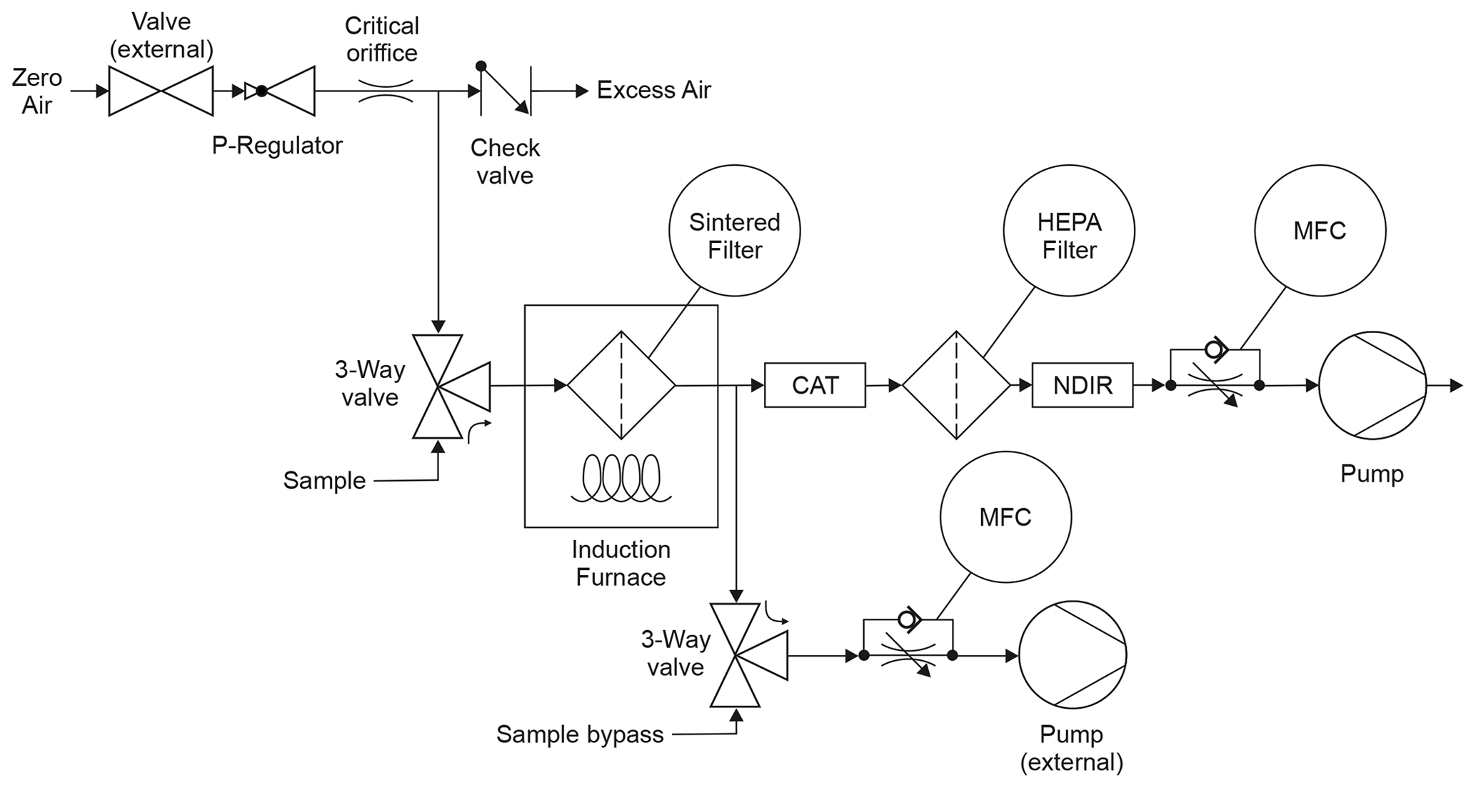
Figure 1 Flow diagram of FATCAT. The instrument has three inlets (zero air, sample and bypass) and three outlets (excess zero air, internal pump and external pump). The three-way valves are actuated together so that either the sample or the bypass inlet is open (sampling mode shown here). The flow of zero air is regulated by means of a pressure reducing valve (P regulator) and a critical orifice. CAT stands for platinum catalytic converter, NDIR is a CO₂ nondispersive infrared sensor, and MFC stands for mass flow controller. Both external components (i.e. the zero air valve and the external pump) are actuated by FATCAT.

FATCAT is built as a stand-alone measurement system, which does not require external laboratory equipment (other than the optional external vacuum pump and denuder). The status data and all relevant parameters can be read through a USB serial interface, which also serves as the link for sending commands. Parameters can also be adjusted and monitored directly at the device through an LCD display accessible throughout a user menu using the interface buttons. The timing of sampling and analysis cycles and data logging are performed by a Raspberry Pi 4B microcomputer (Raspberry Pi Foundation, UK) using software programmed in Python. The software provides a graphical user interface, but the device can also run “headless” using programmed scripts.

During sampling, the instrument opens the sample inlet and closes the sample bypass. In this mode FATCAT gathers an aerosol sample on a sintered hastelloy-X filter (SIKA-HX3; GKN sinter metal filters, Germany). When using only the internal pump, the sampling flow rate can be regulated up to a maximum of 2 L min⁻¹. An external pump can be used for applications that require higher flows rates. In this configuration, the sampling flow rate is constrained by atmospheric pressure, as the sintered filter acts as an ensemble of critical orifices. Notably, the maximum achievable sampling flow rate is typically around 10 L min⁻¹ at the Swiss Plateau (approximate elevation of about 400 m above sea level (m a.s.l.), ambient pressure around 960 mbar) and around 7 L min⁻¹ at the Sphinx Observatory of the Jungfraujoch (situated at 3500 m a.s.l., ambient pressure around 640 mbar). The sample flow throughout the pumps is controlled by two mass flow controllers (MFCs; Vögtlin Instruments, Switzerland).

Conversely, the analysis mode seals the sample inlet and opens the sample bypass and zero air inlets. All experiments described in this article use synthetic air with low carbon dioxide and hydrocarbon content (CO₂≤0.5 ppm, hydrocarbons ≤0.1 ppm; APHAGAZ 1 synthetic air; Carbagas AG, Switzerland) as zero air. It could be possible to use ambient air for the analysis and subtract the CO₂ baseline as described below. Nevertheless, further characterization is needed to determine how this would affect parameters like the limit of detection of the instrument. The analysis mode can also be used instead of the sampling mode in order to gather a blank probe to determine the zero offset and its variability. During sample analysis, the induction furnace is turned on and the filter is heated in less than 1 min, under the zero air atmosphere with a flow rate of 1 L min⁻¹, to a temperature of the order of 800 ^∘C. This temperature is enough to effectively oxidize and desorb carbonaceous material collected during the sampling phase. A platinum catalyst (OST.1700.200.A9; Hug Engineering, Switzerland) positioned downstream of the induction furnace and heated to 200 ^∘C ensures complete oxidation of organic substances and avoids measurement artefacts arising from the incomplete combustion of the sample. This type of catalyst is used for after-treatment of diesel-vehicle emissions, which makes it a very robust and long-living component. A nondispersive infrared (NDIR) carbon dioxide sensor (LI-850; LICOR, Germany) is used for CO₂ quantification. During sample analysis, the flow of zero air through the sintered filter is set to 1 L min⁻¹. Sampling can be restarted once the filter cools down to a predefined temperature. A cooling period of approximately 20 min is typically required to reach a target temperature of 30 ^∘C. The heating of the filter has been optimized through finite element calculations, ensuring uniform and localized heating of the sample. Several pt-1000 sensors monitor the temperature of the sampling filter, the induction coil and the catalyst.

Ideally, the total carbon mass in the sample, m_TC, can be derived from the CO₂ mass concentration, $c_{{\mathrm{CO}}_{\mathrm{2}}}$, and the mass flow rate, f, throughout the instrument using

$$\begin{array}{}\text{(1)}& \begin{array}{l}{m}_{\mathrm{TC}}=\underset{t_{\mathrm{1}}}{\overset{t_{\mathrm{2}}}{\int }}\frac{\mathrm{d}{m}_{\mathrm{TC}}}{\mathrm{d}t}\mathrm{d}t\\ m_{\mathrm{TC}}=\frac{M_{\mathrm{C}}}{M_{{\mathrm{CO}}_{\mathrm{2}}}}\underset{t_{\mathrm{1}}}{\overset{t_{\mathrm{2}}}{\int }}f\left(t\right)\left(c_{{\mathrm{CO}}_{\mathrm{2}}}\left(t\right)-c_{{\mathrm{CO}}_{\mathrm{2}},\mathrm{baseline}}\right)\mathrm{d}t,\end{array}\end{array}$$

where $c_{{\mathrm{CO}}_{\mathrm{2}},\mathrm{baseline}}$ is the CO₂ mass concentration from the zero air, $t_{\mathrm{1}}\le t\le t_{\mathrm{2}}$ is duration of the analysis, and M_C and $M_{{\mathrm{CO}}_{\mathrm{2}}}$ are the molar masses of C and CO₂ respectively. Nevertheless, the heating of the filter causes the filter pores to reduce in size and, as a result, the pressure downstream of the filter will drop. This fast change in pressure is not compensated fast enough by the CO₂ sensor, which results in an offset of the m_TC or a non-zero m_TC for a blank sample. The shift in CO₂ concentration for a blank sample is, however, reproducible. This allows us to calculate a corrected total carbon mass of the sample, $m_{\mathrm{TC}}^{*}$, by subtracting an average blank CO₂ offset curve from the measured CO₂ mass concentration. Equation (1) becomes

$$\begin{array}{}\text{(2)}& \begin{array}{l}{m}_{\mathrm{TC}}^{*}=\underset{t_{\mathrm{1}}}{\overset{t_{\mathrm{2}}}{\int }}\frac{\mathrm{d}{m}_{\mathrm{TC}}^{*}}{\mathrm{d}t}\mathrm{d}t\\ \begin{array}{rl}{m}_{\mathrm{TC}}^{*}& ={\displaystyle \frac{M_{\mathrm{C}}}{M_{{\mathrm{CO}}_{\mathrm{2}}}}}\underset{t_{\mathrm{1}}}{\overset{t_{\mathrm{2}}}{\int }}f\left(t\right)\\ & \left(c_{{\mathrm{CO}}_{\mathrm{2}}}\left(t\right)-c_{{\mathrm{CO}}_{\mathrm{2}},\mathrm{baseline}}-{\stackrel{\mathrm{‾}}{c}}_{{\mathrm{CO}}_{\mathrm{2}},\mathrm{blank},\mathrm{offset}}\left(t\right)\right)\mathrm{d}t,\end{array}\end{array}\end{array}$$

where ${\stackrel{\mathrm{‾}}{c}}_{{\mathrm{CO}}_{\mathrm{2}},\mathrm{blank},\mathrm{offset}}\left(t\right)$ is the average evolution of the CO₂ mass concentration for a blank sample. This parameter can be expressed as

$$\begin{array}{}\text{(3)}& \begin{array}{rl}& {\stackrel{\mathrm{‾}}{c}}_{{\mathrm{CO}}_{\mathrm{2}},\mathrm{blank},\mathrm{offset}}\left(t\right)\\ & ={\displaystyle \frac{\mathrm{1}}{n}}\sum _{i=\mathrm{1}}^n\left[c_{{\mathrm{CO}}_{\mathrm{2}},\mathrm{blank},i}\left(t\right)-c_{{\mathrm{CO}}_{\mathrm{2}},\mathrm{baseline},\mathrm{blank},i}\right],\end{array}\end{array}$$

for n analysed blanks with CO₂ curves $c_{{\mathrm{CO}}_{\mathrm{2}},\mathrm{blank},i}$ and baselines $c_{{\mathrm{CO}}_{\mathrm{2}},\mathrm{baseline},\mathrm{blank},i}$. It is important to include the individual baseline levels of CO₂ in the calculation to account for variations of the zero air composition or long-term drifts of the CO₂ sensor.

The average mass concentration of total carbon, c_TC, after sampling a volume, V, of carrier gas can be calculated from the total carbon mass in the filter as $c_{\mathrm{TC}}=m_{\mathrm{TC}}^{*}/V$. By taking a closer look at Eq. (2), it becomes clear that the measurement span of FATCAT is closely related to the performance of the CO₂ sensor. The limit of detection of the sensor and the length of the integral, together with the already mentioned variations of the CO₂ baseline, will directly affect the limit of detection of FATCAT. On the other end, FATCAT's upper limit of quantification is determined by the upper measurement range of the CO₂ sensor (i.e. nominal limit 20 000 ppm) as well as by the shape of $c_{{\mathrm{CO}}_{\mathrm{2}}}\left(t\right)$. We will show that $c_{{\mathrm{CO}}_{\mathrm{2}}}\left(t\right)$ produces curves that can be interpreted as thermograms. As will be discussed below, homogeneity of carbonaceous species plays a role as homogeneous samples result in narrow thermograms that may surpass the upper range of the CO₂ sensor at lower filter loads compared to heterogeneous samples with wider thermograms.

2.2 Baseline

We performed a series of periodic blank measurements to determine the offset of our system. For this purpose, we used FATCAT to sample ambient aerosol from the exterior of our laboratory with a flow rate of 10 L min⁻¹. The campaign started with a new filter that was exposed to ambient aerosols during the day. The ambient sample was analysed in 1 h intervals. Once a day, after the sample analysis at 23:00 LT, the ambient sample was automatically replaced with a blank measurement as described in the previous section. The purpose of this exercise was to investigate the drift of instrument baseline during its deployment at a measurement site. Drift of the CO₂ sensor as well as other factors like contamination of the instrument and obstruction of the filter may influence the results. Blank measurements are also used to calculate the average offset curve described in Eq. (3). The setup for ambient measurements and examples of measurements at different locations is beyond the scope of this article and will be discussed in a future publication.

2.3 Aerosol generation in the laboratory

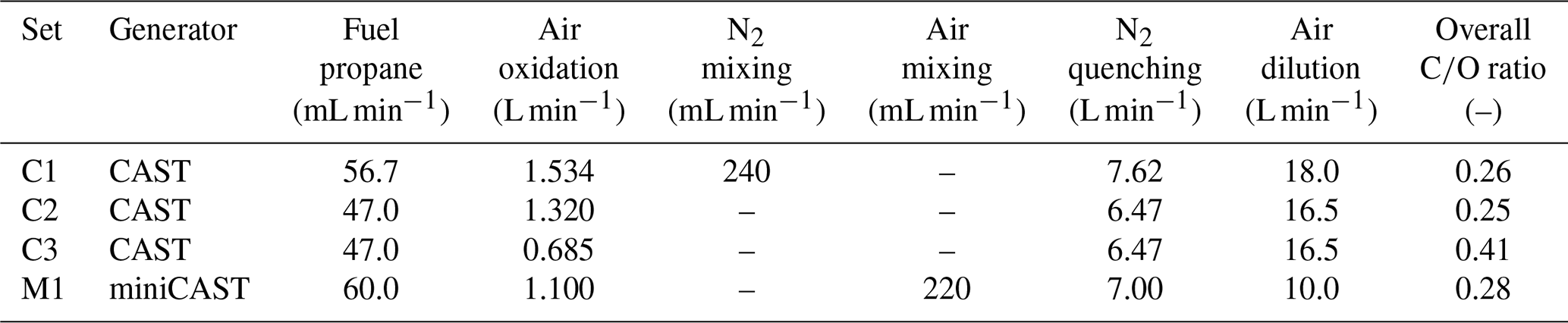
We tested FATCAT using carbonaceous aerosol from a combustion aerosol standard generator (CAST; Jing Ltd, Switzerland). Figure 2 shows a schematic representation of the experimental setup. Two main sets of experiments were performed. The first set of experiments consisted of the aerosol sample directly produced by the generator. The CAST generates aerosol particles using a quenched propane diffusion flame. The fraction of OC and EC in the particles varies depending on the settings, in particular the air-to-fuel ratio during combustion. The second set of experiments consisted of particles with a high EC-to-TC ratio, generated by means of a miniCAST 5201 Type BC (Jing Ltd., Switzerland), which were then coated with different amounts of secondary organic matter (SOM), produced using α-pinene (≥97 % purity, Sigma Aldrich, Switzerland) as a precursor substance, by means of an organic coating unit (OCU; Keller et al., 2022). This set of experiments was performed during a separate campaign. The experimental setup is described in detail by Kalbermatter et al. (2022). The CAST and miniCAST set points used for both campaigns can be found in Table 1. The sample was diluted by means of a homemade rotating disc diluter (Hueglin et al., 1997) using synthetic air as a carrier gas (APHAGAZ 1 synthetic air; Carbagas AG, Switzerland). A three-way valve was used to select between the aerosol sample and the particle-free synthetic air. This was done to ensure that the measurement devices and the sampling filter were exposed to the same concentration of aerosol particles during the same interval of time.

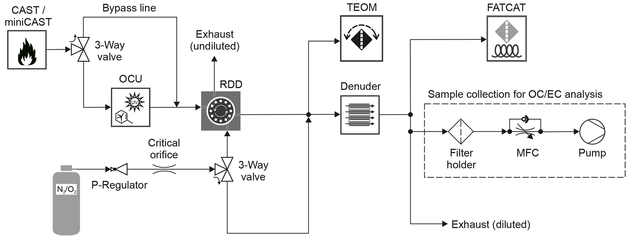
Figure 2 Schematic representation of the setup used for the production and measurement of carbonaceous aerosol. The three-way valves control the coating of the particles (uncoated mode shown) and use delivery of synthetic air (shown in the diagram) or diluted test aerosol to the measurement devices. The boxes represent the following instruments: aerosol generator (CAST/miniCAST), organic coating unit (OCU), rotating disc diluter (RDD), tapered element oscillating microbalance (TEOM) and FATCAT. The flow rate of synthetic air (${\mathrm{N}}_{\mathrm{2}}/{\mathrm{O}}_{\mathrm{2}}$) is regulated by means of a pressure reducing valve (P regulator) and a critical orifice. Denuder stands for activated carbon denuder and MFC for mass flow controller.

Table 1 Set points for the laboratory generated carbonaceous sample. CAST stands for the combustion aerosol standard generator (Jing Ltd, Switzerland) model CAST-00-4, whereas miniCAST stands for the model miniCAST 5201. The set M1 was used during the coating experiments described by Kalbermatter et al. (2022). $\mathrm{C}/\mathrm{O}$ ratio refers to the air-to-fuel mixture during combustion and not to the elemental composition of the produced aerosol.

2.4 Characterization of laboratory samples

A tapered element oscillating microbalance (TEOM model 1405; Thermo Fisher Scientific Inc., USA) with a flow rate of 1.5 L min⁻¹ was used to measure the mass concentration of the sample. The temperature of the TEOM sampling head was set to 50 ^∘C for samples C1 through C3 and to 30 ^∘C for the M1 samples of the coating experiments to minimize the desorption of coating material. The oscillating frequency of the microbalance was logged by a computer every 10 s throughout serial connection. The mass increment of the oscillating element was calculated using this frequency and the calibration constant of the TEOM as described by the user's manual. On a sampling line parallel to the TEOM, an active charcoal denuder (Part. No. M3456; Aerosol d.o.o., Slovenia) was used to remove gas-phase species to avoid positive sampling artefacts. This procedure was not applied to the TEOM as its filter is heated. Aerosols were collected downstream of the denuder by FATCAT at a rate of 1.5 L min⁻¹ and on quartz-fibre filters (filter diameter 47 mm) at a rate of 1 L min⁻¹ for TOT analysis using the EUSAAR2 protocol. Samples from the coating experiments were collected in QR-100 quartz-fibre filters (Advantec, Japan) and analysed by the Swiss Federal Institute of Metrology (METAS), whereas the rest of the samples were collected in Pallflex Tissuquartz 2500QAT-UP filters (Cytiva, USA) and analysed by a commercial laboratory (Particle Vision GmbH, Switzerland). The TOT analysis returns the OC and EC concentration per square centimetre of the sample, divided into different subfractions. The total amount of OC, EC and TC captured in the filter can be calculated from these fractions. The data from the TOT analysis were adjusted for flow rate and filter surface for comparison against the TC measurements from FATCAT.

2.5 Biomass-burning samples

We performed a set of experiments with biomass-burning samples in order to challenge FATCAT with high loads of an aerosol with variable, not entirely carbonaceous composition. The tests were performed according to the EN 16510:2018 standard series for residential solid fuel-burning appliances at the certified biomass combustion test bench of our partner institute of bioenergy and resource efficiency FHNW. Beech wood was used throughout all experiments. The tests were complemented with our own measurements of TC using FATCAT and filter collection for thermal–optical analysis following the procedure described by Keller and Burtscher (2017). Shortly, a partial flow was taken from the stack and diluted at a factor 1:4 using zero air at a temperature of 200 ^∘C. The purpose of this dilution is to avoid condensation of water once the sample cools down at room temperature. The diluted flue gas is then cooled down to room temperature and aged by means of an oxidation flow reactor (i.e. the micro smog chamber, MSC; Keller and Burtscher, 2012) in order to promote the formation of secondary organic aerosols. Samples for TOT analysis are gathered downstream of the MSC. We modified the original setup to include sampling by FATCAT in parallel to the TOT samples. The flow through the MSC was held at a rate of 1 L min⁻¹, but the sample was diluted using additional zero air downstream of the MSC. The goal was to create a total of 4 L min⁻¹, which could then be sampled in parallel by FATCAT and on a quartz-fibre filter. The quartz filters for TOT analysis sampled emissions using a flow rate of 1 L min⁻¹, whereas flows of 1, 2 or 3 L min⁻¹ were used to collect samples in FATCAT. This was done in order to challenge the instrument with high filter loads. Here as well, the results from the TOT analysis were adjusted for flow and filter area to compare them against FATCAT.

Table 2 shows characteristics of the stoves selected for the experiments. The first one is a modern, certified stove for cooking and baking. The second one is an old stove model that has been discontinued by the manufacturer. Three cycles were performed each measurement day. We measured the first cycle of the day (i.e. cold cycle), which was then followed by two immediate warm refuelling cycles. Each cycle takes approximately 40 min. We only measured the second warm cycle due to the 20 min recovery time need for the FATCAT filter to reach 30 ^∘C.

Table 2 Specifications of the two batch-operated wood-burning appliances used for this study.

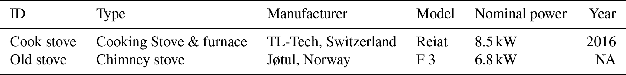
NA: not available. kW stands for kilowatts.

3 Results and discussion

3.1 Long-term behaviour of the baseline

Figure 3 shows the result of a periodic, once a day, blank measurement for a total of 109 d, where the FATCAT sampled and analysed zero air. The purpose of this exercise was to determine the long-time stability of the system. NDIR sensors, like the one used by FATCAT, are very precise in the short term but suffer from offset drifts over extended time periods. Nevertheless, for the purpose of our measurements, we only require the CO₂ signal to be stable for less than 120 s. The CO₂ concentration in the zero air, measured before the start of the analysis, builds the baseline for the measurement. Still, factors like ambient pressure and temperature, contamination of the sampling lines with organic material, or deterioration of the filter could affect the long-time performance.

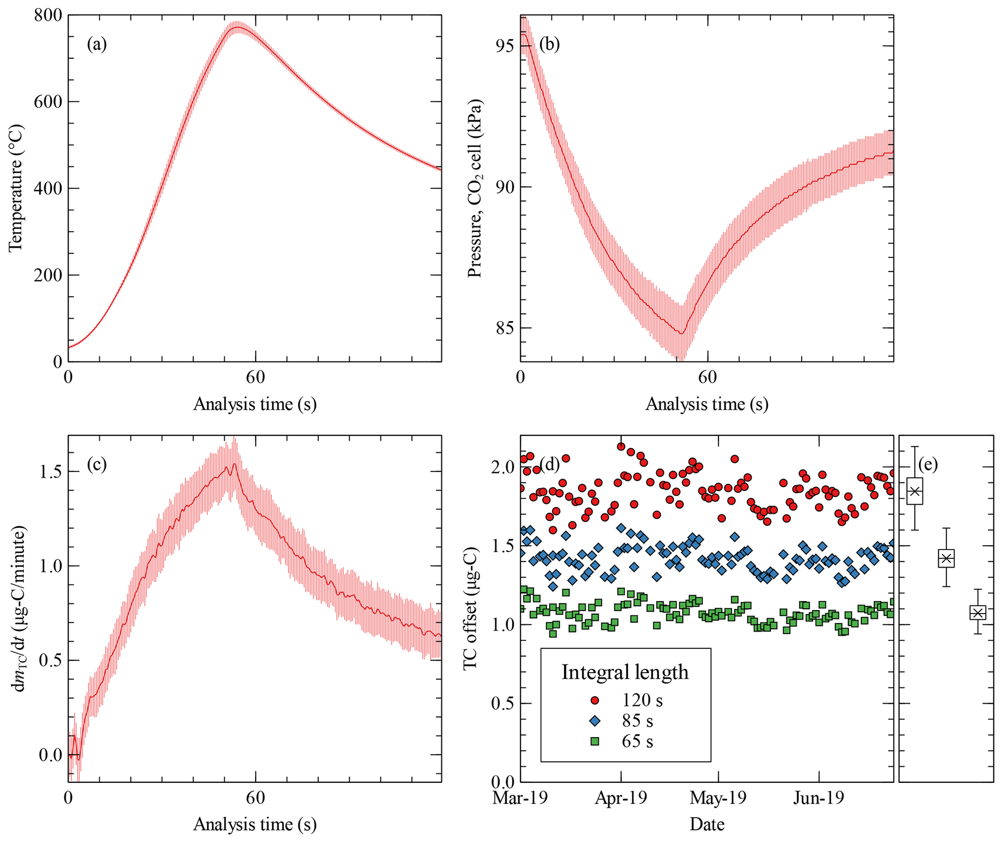
Figure 3 Evaluation of the instrument response during the analysis of 109 consecutive blank samples measured once a day for almost 4 months. Average curve (dark red line) with error bars (standard deviation, light red) for the evolution during the analysis cycles of (a) the temperature measured downstream of the sampling filter, (b) pressure in the CO₂ sensor cell, and (c) differential total carbon offset. Time zero marks the start of the heating of the filter. (d) The time evolution of the determined offsets in total carbon, i.e. the area under the curve of individual blank measurements that built figure (c), and the boxplot representation of the whole series (e) calculated from the integral of the individual blank samples for different integration lengths, starting at time zero of the analysis cycle. µg-C stands for micrograms of carbon.

The curves presented in Fig. 3a and b show that the evolution of temperature and pressure was very reproducible during this prolonged campaign. The temperature evolution affects how the sample will be released by combustion or desorption from the filter, whereas the pressure affects the optical measurement of the CO₂ concentration. The increase in pressure drop is caused by the reduction of the pore size due to the expansion of the metal of the filter during heating. Ideally, this change in pressure would be compensated by the correction algorithm of the CO₂ sensor. A constant CO₂ concentration would result in a constant CO₂ signal independent of the pressure drop, Nevertheless, Fig. 3c shows that this is not the case as the differential TC signal diverges from the zero line for the zero air measurement. This is most likely caused by a pressure compensation of the CO₂ sensor that is too slow, which is design for ambient conditions where fast changes in pressure are not expected. We are considering accessing the raw extinction signals from the CO₂ and constructing our own correction algorithm or contacting the manufacturer for an original equipment manufacturer (OEM) solution for a future optimization of our measurement system.

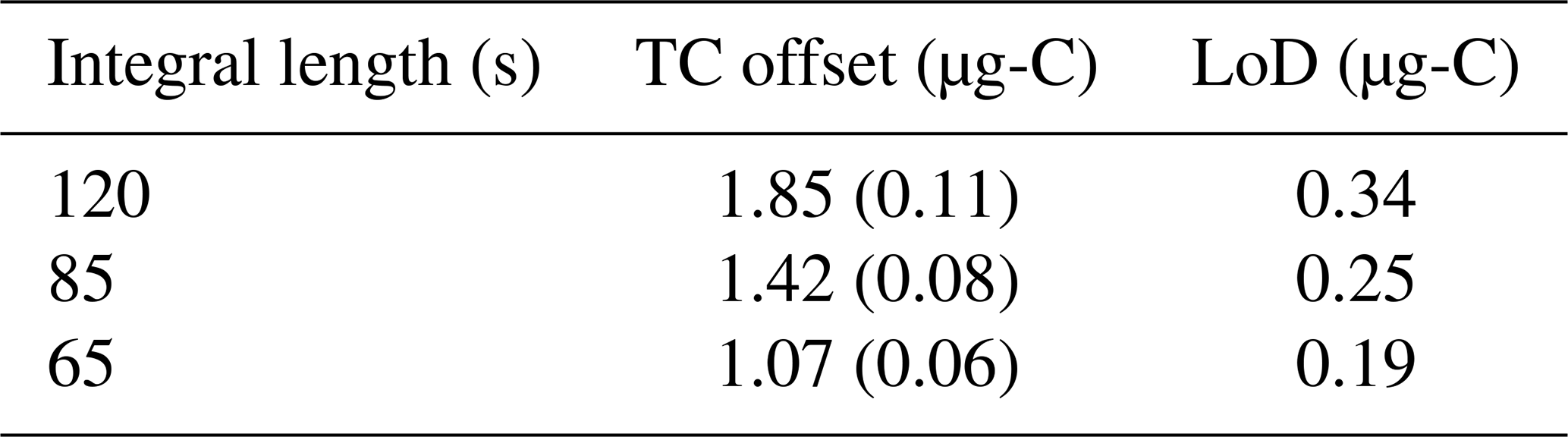
The offset of the total carbon signal of individual blank measurements (Fig. 3d) is calculated by integrating the evolution of total carbon, dm_TC, according to Eq. (1). As discussed, the integral of a blank sample is non-zero due to the pressure drop in the CO₂ sensor. Longer integration times cause larger offset (Fig. 3d and e and Table 3) and a more dispersed data. Thus, an optimal limit of detection can be achieved by choosing the shortest possible integration time that still captures the total carbon information from the sample. In our experience, an integration time of 65 s is enough for an ambient sample even at an urban location. The corresponding limit of detection would be TC =0.19 µg-C (micrograms of carbon) sampled in the filter. This translates to an average ambient concentration of TC = 0.32 and 0.16 µg-C m⁻³ for 1 or 2 h of sampling, respectively, using a flow rate of 10 L min⁻¹. Lower limits of detection can be achieved through longer sampling periods or, if possible, by using a higher sample flow rate.

Table 3 Offset of the average, uncorrected, blank sample from the data shown in Fig. 3 for three different integration lengths. The standard deviations are shown in parentheses. LoD is the corresponding limit of detection calculated from the noise-to-background using the 3σ criterion. µg-C stands for micrograms of carbon.

3.2 Concentration-response analysis

Figure 4a shows a comparison between the aerosol mass measurement by the TEOM and the total carbon mass measured by FATCAT. Samples C1 and C2 were produced by the CAST with a lean flame composition, with an air-to-fuel mixture of $\mathrm{C}/\mathrm{O}$ = 0.26 and 0.25 respectively, which results in particles with a high elemental carbon fraction of $\mathrm{EC}/\mathrm{TC}$ = 0.91 (see Table 4). There is an extremely good correlation (R²=0.999) between these two instruments based on very different measuring principles. The TEOM measures mass based on the change of the oscillation frequency of a mass transducer and is independent of the particle composition. The slope of the correlation, m, indicates that the sample has a carbon mass fraction of $f_{\mathrm{C}}=m=\mathrm{0.94}$. This compares well with the values of f_C=0.90 and 0.93 reported for other flame generators (Corbin et al., 2020) and the values of $\mathrm{0.90}\le f_{\mathrm{C}}\le \mathrm{0.98}$ quoted in that article for other literature studies. The inset in Fig. 4a shows the third sample, C3, which was produced with a rich flame ($\mathrm{C}/\mathrm{O}$ = 0.41), which increases the OC fraction in the aerosol. The correlation between FATCAT and the TEOM is also extremely good (R²=0.993). However, the intercept is shifted from zero, and the slope of the curve is steeper than for the C1 and C2 samples. The latter is unexpected given that OC is not exclusively composed of carbon. A positive artefact from the TEOM, due to the retention of gas phase organic species from the non-denuded sample, could cause the displacement of the intercept. Similar behaviour has been demonstrated through a comparison of denuded and non-denuded samples (Subramanian et al., 2004). The TEOM minimizes positive sampling artefacts by heating the sampling filter to a standard temperature of 50 ^∘C; this targets humidity and may even cause negative artefacts from the most volatile fraction of OC. However, this temperature may not be enough to prevent the adsorption of gas-phase OC from the C3 sample, which contains mainly species detected during the OC3 step (i.e. desorption at 450 ^∘C under a helium atmosphere) of the TOT analysis (Fig. 4c). A negative artefact from the side of FATCAT cannot be discarded but is less likely to happen due to the low volatility of the OC3. Additionally, a negative artefact would not explain the displacement of the intercept, as the artefact would be more pronounced at higher filter loads due to the longer sampling time required to achieve them. This would result in a less pronounced slope for this sample.

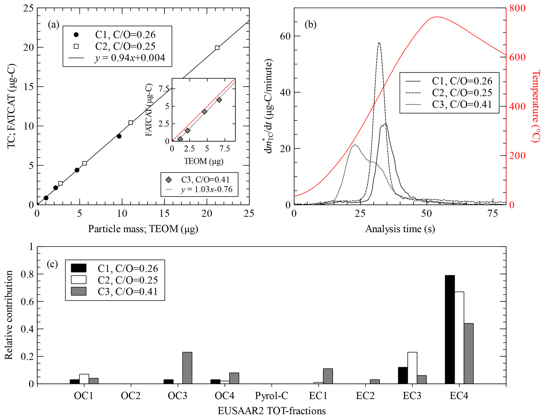
Figure 4 (a) Total carbon measured by FATCAT against particle mass deposited in the TEOM for three different propane flame aerosol samples. The line shows a linear fit to the C1 and C2 samples (coefficient of determination, R²=0.999). The inset shows the third sample, C3, a linear fit (R²=0.993), and the 1:1 line (dashed lines). (b) Blank-corrected fast thermograms for the three types of propane flame samples. Samples with a similar total carbon mass were selected for this comparison, i.e. TC =5.2 µg-C, TC =4.4 µg-C and TC =5.6 µg-C for C1, C2 and C3 respectively. The red line shows the temperature measured behind the filter during the analysis process. (c) Relative carbon mass contributions to the analysis steps of the thermal protocol EUSAAR2 for the three samples. OC1 through OC4 are the organic carbon fractions, Pyrol-C is the pyrolysed organic carbon, and EC1 through EC4 are the elemental carbon fractions. $\mathrm{C}/\mathrm{O}$ refers to the air-to-fuel mixture used to produce the sample.

Table 4 Properties of the propane flame aerosol samples. The M1 samples correspond to the aerosol generated and described by Kalbermatter et al. (2022) as set point 0.1. The uncertainty of the $\mathrm{EC}/\mathrm{TC}$ is based on the uncertainties given by the instrument's software, calculated as the detection limit of 0.2 µg-C cm⁻² plus 5 % of the carbon mass determined in the analysis for each carbon fraction.

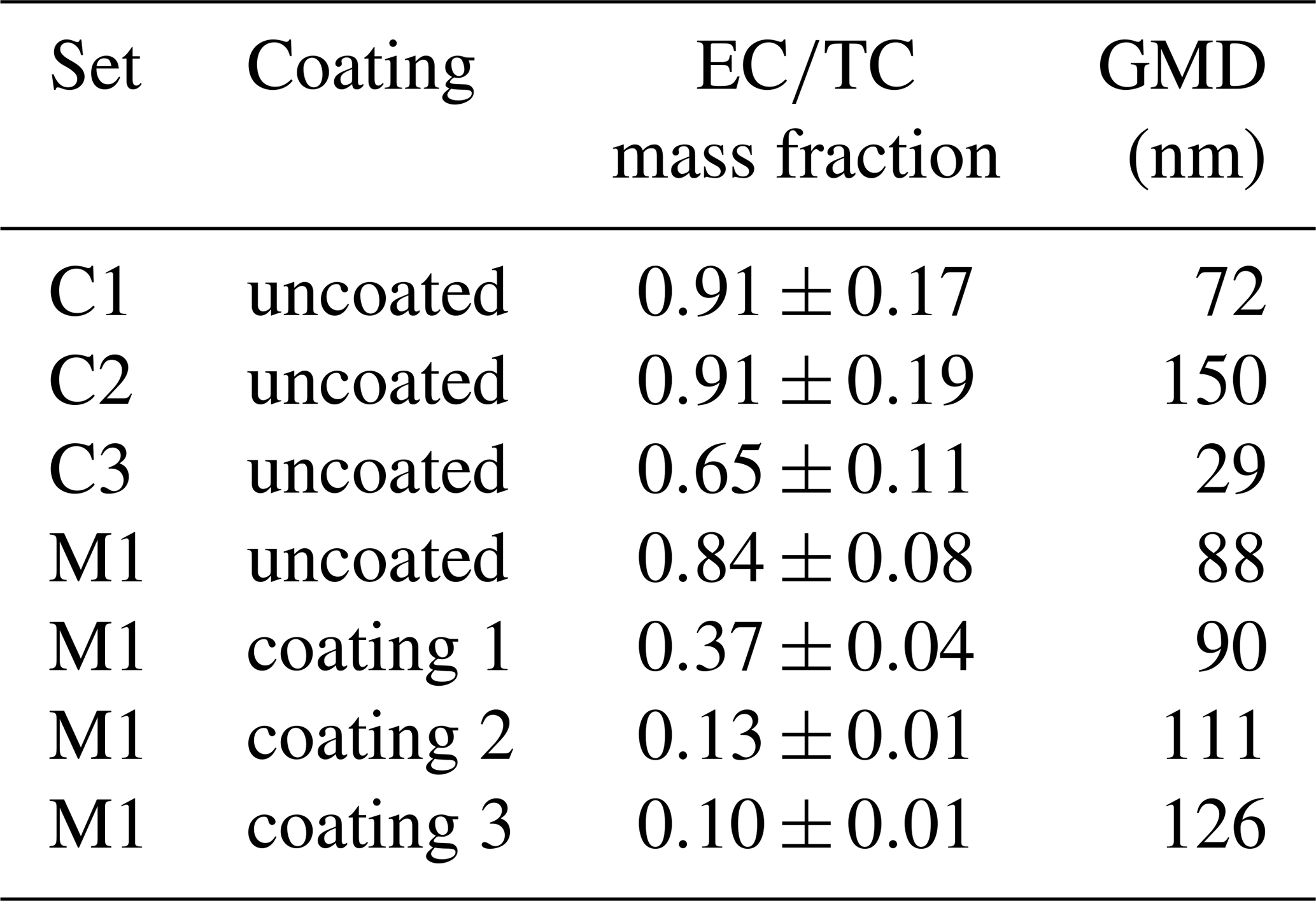
The induction-based flash-heating furnace of FATCAT allows for a direct, fast and homogeneous heating of the filter. This type of heating produces reproducible CO₂ signal patterns that depend on the sample composition and, thus, can be used to extract information beyond TC quantification. We refer to them as fast thermograms. Nevertheless, as opposed to thermograms produced by thermal–optical methods, there is neither a heating protocol based on predefined temperature steps nor a split between EC and OC using different gases. Figure 4b shows the thermograms for the C1 through C3 samples. Samples C1 and C2 were produced with similar air-to-fuel mixing ratios, have a comparable $\mathrm{EC}/\mathrm{TC}$ fraction and are also very similar in terms of the OC and EC subfractions from the TOT analysis (Fig. 4c). Sample C3 was created with a richer flame and has a higher OC fraction ($\mathrm{OC}/\mathrm{TC}$ = 0.35). The EC fraction evolves later in the analysis, at higher filter temperatures, than the OC fraction. The two samples with high $\mathrm{EC}/\mathrm{TC}$ (i.e. C1 and C2) create different patterns even though they were created with similar air-to-fuel mixtures. C2 appears to be more homogeneous. It has a narrow and well-defined distribution. The main difference between the samples is the residence time in the flame before quenching, which was shorter in the case of C1 compared to C2. This leads to smaller particles with geometrical mean diameter (GMD) = 72 and 150 nm for C1 and C2 respectively. Soot formation models suggest that variations in both particles size and flame carbon-to-oxygen have an effect in the degree of maturity of soot particles (Kelesidis and Pratsinis, 2019b). This has been validated for particles from the CAST generator (Kelesidis et al., 2017, 2021). Mature soot particles have smaller oxidation rates than more nascent ones, as they contain less hydrogen (see, e.g. Kelesidis and Pratsinis, 2019a; Maricq, 2014). This difference may explain the broadening and shift of the thermograms.

Figure 5 shows the results from the coating experiment. We start with an uncoated seed aerosol (M1) sample with an elemental carbon fraction $\mathrm{EC}/\mathrm{TC}$ = 0.84 and a size distribution with GMD = 84 nm. The particles are gradually coated in three steps (coatings 1 through 3) by SOM from the ozonolysis of α-pinene. The particle size increases due to the addition of organic mass (OM) up to GMD = 126 nm, while the elemental carbon fraction is reduced to $\mathrm{EC}/\mathrm{TC}$ = 0.1. Here again, the carbonaceous fraction of the coating material can be inferred from the slope of the linear regression between TEOM and FATCAT (Fig. 5a) to f_C=0.56. The inverse of f_C indicates that the coating material has a ratio of $\mathrm{OM}/\mathrm{OC}$ = 1.79. This is in excellent agreement with the range of $\mathrm{1.78}\le \mathrm{OM}/\mathrm{OC}\le \mathrm{1.85}$ reported for α-pinene SOM produced using a similar setup (Leni et al., 2022, the Supplement). Other oxidation states, leading to diverse $\mathrm{OM}/\mathrm{OC}$, are also possible (see, e.g. Cain et al., 2021). In our case, OC1 is the predominant organic carbon fraction (Fig. 5c). This step corresponds to the most volatile fraction of the thermal–optical analysis, performed at 200 ^∘C under a helium atmosphere. Nevertheless, there is also additional material in all the other organic carbon analysis steps, which speaks for a diversity of organic species. The concentration of seed particles and, thus, the amount of EC was kept constant throughout the different coating steps. The fast thermograms (Fig. 5b) show that, for these internally mixed particles, the organic material adds an independent feature at lower temperatures in the thermogram without affecting the shape of the contribution of the uncoated seed. This is not obvious as the organic material causes the cores to collapse during coating (Keller et al., 2022), which in turn could have affected the thermogram feature corresponding to the particle core.

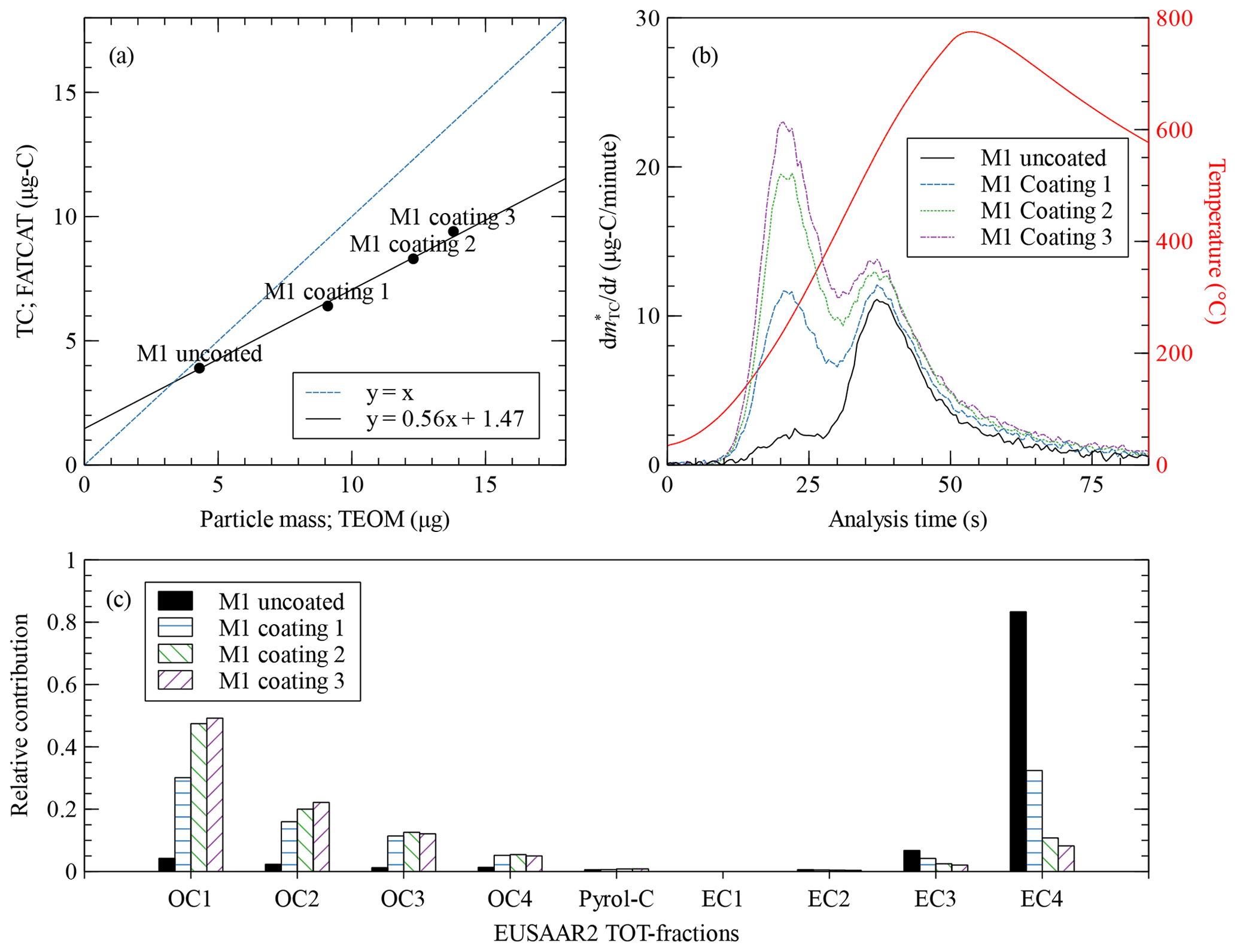
Figure 5 (a) Total carbon measured by FATCAT against particle mass deposited in the TEOM for the uncoated soot sample M1 and the three different coated samples. The solid line shows a linear fit to the four data points (coefficient of determination, R²=0.996). The concentration of the seed aerosol was kept constant for all samples. Thus, the increase in mass comes from organic coating. This causes the data points to deviate increasingly from the 1:1 line (dashed line), as only a fraction of the mass of organics comes from the carbon atoms. (b) Blank-corrected fast thermograms for the uncoated soot and the three coating levels. The red line shows the temperature measured behind the filter during the analysis process. (c) Relative carbon mass contributions to the TOT analysis steps of the EUSAAR2 protocol for the uncoated aerosol and the coated samples. OC1 through OC4 are the organic carbon fractions, Pyrol-C is the pyrolysed organic carbon, and EC1 through EC4 are the elemental carbon fractions.

3.3 Biomass-burning emissions

Figure 6 shows the results of measurements of emissions from two wood-burning stoves during type approval testing. As opposed to the propane flame aerosol from the CAST, the composition of the wood-burning samples is not so easily controllable and therefore difficult to reproduce. It depends on the combustion technology and can also have a great degree of variability for samples from a single appliance (see, e.g. Lamberg et al., 2011). Wood-burning emissions are composed of OC, EC and non-carbonaceous inorganic materials like ashes and salts. The propane flame examples described in this article use low mass loads, which are relevant for ambient monitoring. The current example demonstrates that FATCAT is capable of measuring mass loads in the hundreds of micrograms of carbon. The analysis of the highest filter load of TC = 554 µg-C caused a brief CO₂ concentration exceeding the CO₂ sensor's quantification limit. This may be considered a worst-case upper detection limit as the wood-burning samples in this study produced narrow fast thermograms.

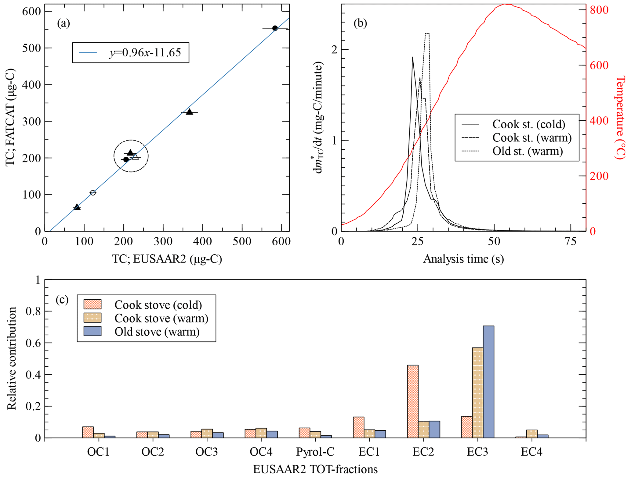
Figure 6 (a) Total carbon measured by FATCAT against the equivalent, filter-size- and flow-corrected, total carbon from the TOT analysis for wood-burning emissions. Triangles and circles correspond to samples from the cooking stove and the old stove respectively. Open and filled symbols correspond to the cold start and warm start tests respectively. The line shows a linear fit to the experimental data. The three points inside the circular region were selected for comparison in the two following graphs of the figure. The error bars of the TOT analysis are based on the uncertainties given by the instrument. (b) Fast thermograms, not blank-corrected, for three samples with similar TC. “Warm” means that the data correspond to a warm cycle of the stove (i.e. a refuelling experiment), whereas “cold” data correspond to the first heating cycle of the day. The curves are less smooth compared to other figures because the data come from an earlier stage of the prototype with coarser data resolution. The red line shows the temperature measured behind the filter during the analysis process. (c) Relative carbon mass contributions to the TOT analysis steps of the EUSAAR2 protocol for three selected samples. OC1 through OC4 are the organic carbon fractions, Pyrol-C is the pyrolysed organic carbon, and EC1 through EC4 are the elemental carbon fractions.

The comparison against the standard TOT analysis shows an excellent correlation for TC (R²=0.996) for data from two different appliances and two test conditions (i.e. cold and warm start test). The fast thermograms and the details of the TOT fractions (Fig. 6b and c) show the diversity of the samples. EC is the main component, but it evolves differently during analysis, mostly during the EC2 (550 ^∘C) step for the first sample (i.e. cooking stove, cold start) and on EC3 (700 ^∘C) for the other two (i.e. cooking stove and old stove, warm start). On the other hand, EC from the propane flame samples has higher refractor temperatures and evolved mainly during the final EC4 step (850 ^∘C). The fast thermograms follow this trend and present further nuances. The cold start sample is the first to evolve ($max\mathrm{d}{m}_{\mathrm{TC}}^{*}/\mathrm{d}t$ at t=23 s), followed by the warm cycle of the cooking stove ($max\mathrm{d}{m}_{\mathrm{TC}}^{*}/\mathrm{d}t$ at t=26 s) and finally the warm cycle of the old stove ($max\mathrm{d}{m}_{\mathrm{TC}}^{*}/\mathrm{d}t$ at t=28 s). EC from propane flame samples evolved even later in the analysis ($max\mathrm{d}{m}_{\mathrm{TC}}^{*}/\mathrm{d}t$ at t=34, 32 and 37 s for C1, C2, and M1 respectively). In turn, the organics from the coating experiments evolve at lower temperatures (i.e. organics peak at t=20.5 s for M1 coatings 1 through 3) than the wood-burning samples. C3 shows a special situation, with two peaks that are close together. The first one, with a maximum at t=23 s, may be a combination of the OC3, OC4 and EC1 components. The time corresponding to the maximum of the second C3 peak cannot be extracted without further analysis, but it is located at t≈30 s and corresponds most likely to the EC4 component. Similar to the propane flame samples, the fast thermograms of the wood-burning samples have different degrees of homogeneity, which in turn suggests further differences in composition.

These examples show that fast thermograms contain more information than a simple quantification of TC. The temperature profile is related to volatility and refractoriness of the sample components. Furthermore, they are reproducible and filter-load-independent. A coating process, which also affects the structure of the seed particle, adds a new component to the thermogram without affecting the signal from the uncoated seed. Nevertheless, there are no discrete steps like the ones defined by thermal–optical protocols. This poses a new challenge for the interpretation and comparison of the data, especially because fast thermogram features from different samples can be partially overlapping (see, e.g. Fig. 4b). This is to be expected since carbonaceous aerosol is collection of very diverse substances with a continuum of physical and chemical properties. Conversely, we are not defining a discrete separation in large arbitrary groups which, like the ones from the thermal–optical methods, fail to provide a clean separation of molecular components (Diab et al., 2015). It has not yet been conclusively investigated how much information about the composition can be obtained from the fast thermograms. What is certain is that they offer a reliable and cost-effective way of obtaining more knowledge about real samples containing carbon.

4 Conclusions

We developed a novel method for the quantification and characterization of carbonaceous aerosol based on the measurement of total carbon. Our prototype uses a rigid metallic filter to capture an aerosol sample, which is then analysed by heating the filter through induction to a temperature around 800 ^∘C in less than a minute under an oxidizing atmosphere. This is long enough to desorb and/or oxidize all the carbonaceous material of the sample. Full oxidation to carbon dioxide is achieved downstream of the filter by means of an oxidation catalyst. Quantification is performed by means of a carbon dioxide NDIR sensor. The components selected for this prototype address several downsides of other measurement systems for TC. In particular, the metallic filter allows for continuous measurement without filter replacement for long periods of time and avoids artefacts caused by, for example, leakage, displacement or damage of the sampling filter. The catalyst, in turn, prevents underestimation of the carbonaceous content of the organic fraction due to incomplete oxidation. This combination of components is, to the best of our knowledge, unique to our system. We still have not determined the typical operation time before filter replacement is needed. Our current configuration has been tested for more than 2 years of continuous operation, sampling ambient aerosol at different locations in the Swiss Plateau, without showing signs of degradation. This may be different for other locations. In any case, filter replacement can be programmed as a standard procedure when replacing other components like the lamp of the NDIR sensor.

The limit of detection of the prototype in terms of filter load is LoD = 0.19 µg-C. In terms of ambient concentrations, this translates to a LoD = 0.32 or 0.16 µg-C m⁻³ for a 1 and 2 h of sampling at 10 L min⁻¹ respectively. Thus, the method is also suitable for continuous TC measurement in our environment. In a future publication, we will report on several months of use at various locations (urban to high alpine) in Switzerland. The upper limit of the measurement technique is set by the upper range of the CO₂ sensor and is higher for heterogeneous samples than for homogeneous samples. We have currently successfully measured filter loads up to TC = 554 µg-C. FATCAT was validated against aerosol mass measurements using TEOM and against TC from TOT analysis. Experiments carried out with standard laboratory-generated samples and batch-operated wood-burning stoves' emissions displayed a high level of correlation between these methods. We also demonstrate that the combination of TC calculated using FATCAT with measurements of aerosol mass can serve as a technique for evaluating the carbonaceous fraction, f_C, of aerosol samples.

Another unique feature of our system is the generation of fast thermograms that contain information about the volatility and refractoriness of carbonaceous particles. Components like SOM, primary OC and soot evolve at different times during the analysis. This is analogous to thermograms generated through thermal–optical methods but without imposing an artificial separation of the carbonaceous material into arbitrary subfractions and without the need for different analysis gases. Samples from wood-burning emissions or propane flame soot that would appear in the same subfraction of a thermal–optical analysis can be distinguished through additional nuances in the fast thermograms. This feature will be studied further with a long-term employment of FATCAT for ambient air monitoring, where fast thermograms contain information about the aerosol composition which could be used for source apportionment studies.