On the potential of the Cluster Ion Counter (CIC) to observe local new particle formation, condensation sink and growth rate of newly formed particles

The Cluster Ion Counter (CIC) is a simple three-channel instrument designed to observe ions in the electrical mobility equivalent diameter range from 1.0 to 5 nm. With the three channels, we can observe concentrations of both ion clusters (sub-2 nm ions) and intermediate ions. Furthermore, as derived here, we can estimate condensation sink (CS), intensity of local new particle formation, growth rate of newly formed particles from 2 to 3 nm and formation rate of 2 nm ions. We compared CIC measurements with those of a multichannel ion spectrometer, the Neutral cluster and Air Ion Spectrometer (NAIS), and found that the concentrations agreed well between the two instruments, with correlation coefficients of 0.89 and 0.86 for sub-2 nm and 2.0–2.3 nm ions, respectively. According to the observations made in Hyytiälä, Finland, and Beijing, China, the ion source rate was estimated to be about two to four ion pairs cm⁻³ s⁻¹. The new CIC is a simple and cheap instrument that can be used in different environments to obtain information about small ion dynamics, local intermediate ion formation and CS in a robust way when combined with the theoretical framework presented here.

1 Introduction

New particle formation (NPF) is the dominant source of the number concentration of aerosol particles in the global atmosphere (Gordon et al., 2017), thereby having potentially large influences on global climate (e.g., Boucher et al., 2013) and regional air quality (e.g., Guo et al., 2014; Kulmala et al., 2022). During the past 2–3 decades, atmospheric NPF has been characterized in terms of the particle formation and growth rates at a vast variety of sites in different atmospheric environments (Wang et al., 2017; Kerminen et al., 2018; Nieminen et al., 2018; Chu et al., 2019; Bousiotis et al., 2021). Such characteristics describe mainly regional NPF, i.e., NPF averaged over relatively large spatial scales of at least tens of kilometers. Much less information is available about local NPF or about the small-scale variability of regional NPF (Kulmala et al., 2024a, b). Such information would be important in identifying hot spot areas for atmospheric NPF or estimating the relative importance of various local sources to regional NPF.

Atmospheric cluster ion (diameters below 2 nm) measurements can provide insight into ion source processes, such as the ion production rate associated with different atmospheric ionization pathways, and into ion loss processes, such as ion–ion recombination or scavenging of ions by a pre-existing atmospheric aerosol population (e.g., Hirsikko et al., 2011; Kontkanen et al., 2013). Observations of intermediate ions (diameters between 2 and 7 nm) can be used to get information about atmospheric NPF (e.g., Tammet et al., 2014), whereas small intermediate ions (approx. 2.0–2.3 nm) can be used to detect “local” NPF, i.e., NPF taking place within a close proximity of a measurement site (Tuovinen et al., 2024).

Intermediate ions are sensitive to both occurrence and intensity of atmospheric NPF (e.g., Horrak et al., 1998; Tammet et al., 2014; Leino et al., 2016). Recently, Kulmala et al. (2024a) and Tuovinen et al. (2024) found that the smallest sizes of intermediate ions describe the local production of new aerosol particles relatively well. These results were obtained using the Neutral cluster and Air Ion Spectrometer (NAIS; Mirme and Mirme, 2013). The NAIS is, however, a sophisticated instrument that provides information not necessarily needed when investigating local NPF, such as detailed knowledge of both ion and particle number size distributions.

In this study, we will analyze data obtained using the Cluster Ion Counter (CIC; Mirme et al., 2024), a recently developed and simple three-channel instrument, and will investigate how this instrument can be utilized to determine several variables important to NPF and small ion dynamics. Our main objectives are to derive simple equations for characterizing ion dynamics related to local NPF and to find out whether the CIC is sensitive and reliable enough for such purposes. In order to reach these objectives, we will first derive equations that can be used to estimate condensation sink (CS), growth rate of newly formed particles and formation rate of 2 nm ions, quantifying the intensity of local new particle formation (actually local intermediate ion formation, LIIF), based on CIC measurements. Next, we will compare ion concentrations between the CIC and NAIS, as measured at the SMEAR II station in Hyytiälä, Finland. Finally, we will demonstrate how to apply CIC measurements in practice for obtaining information about local NPF and related quantities, including the condensation sink.

2 Material and methods

2.1 Cluster Ion Counter (CIC)

The Cluster Ion Counter (CIC) is an instrument for measuring the total number concentration of both positive and negative cluster ions. The CIC uses two separate first-order cylindrical differential mobility analyzers, one for each polarity (Tammet, 1970). The principal components of the analyzers are a central electrode on the axis of the analyzer that is held at a steady voltage and three cylindrical collecting electrodes flush with the outer wall of the analyzer which are at zero electric potential. A constant sample flow is produced through the analyzer using a blower at the outlet. The sampled ions passing through the analyzers are repelled by the central electrode, and they may deposit on one of the collecting electrodes depending on the electrical mobility of the ions. The electric current produced by the deposited ions is measured using high-precision integrating electrometers (Mirme et al., 2024).

The mobility-dependent detection efficiency curves of the three channels are determined by the geometry of the analyzer, the sample air flow rate and the electric voltage of the central electrode. According to the idealized model of differential mobility analyzers (Tammet, 1970), the primary parameters governing the detection efficiency curves and the limiting mobilities of the collecting electrodes are the electrical capacitances between the central electrode and the each collecting electrode, as well as the ratio of the sample flow rate to the central electrode voltage. The original CIC was designed to allow the estimation of average cluster ion mobility. However, the device can easily be modified to focus on other aspects of the mobility distribution.

In the CIC, the ratio of the flow rate to the voltage can be freely adjusted through software. The lengths of the collecting electrodes and geometry of the central electrode of the CIC can be changed without requiring additional modifications to the device.

A modified analyzer for the CIC was developed to estimate the concentration of intermediate ions roughly between 2.0 and 2.3 nm. Due to the relatively simple construction of the CIC, and specifically the absence of a separate sheath air flow layer in the mobility analyzer, the detection efficiency curves of the individual electrodes of the CIC are relatively wide and extend far towards larger particles (Fig. 1). However it is notable that for particles beyond certain size the transfer functions differ only by a constant coefficient. We can use the signal from one channel to compensate for the concentration of larger particles in another channel and virtually achieve a higher size resolution.

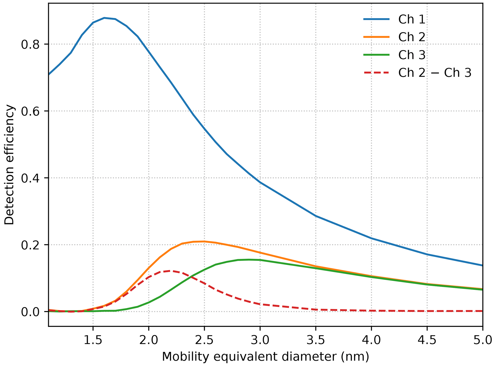
Figure 1 Experimental detection efficiency for ions in the range from 1.1 to 5.0 nm for each of the three collecting electrodes of the CIC. Due to the absence of a separate sheath air flow layer in the mobility analyzer, the detection efficiencies do not have a sharp upper size limit; instead, they asymptotically approach zero as particle size increases. Ion concentrations in a narrower size range can be estimated by subtracting the signal of channel 3 from channel 2. The detection efficiencies of the two channels converge from 2.5 to 3.5 nm and are practically equal for larger particles.

We altered the collecting and central electrode geometry, as well as voltage, and flow rate within the mechanical constraints of the original device so that the transfer functions of channel 2 and 3 would differ only in a relative narrow size range and the difference would peak between 2.0 and 2.3 nm. This required extending the first collecting electrode and shortening the second and third electrode, as well as changing the diameter and length of the central electrode.

In the modified CIC, the signal from the first electrometer can be used to estimate the cluster ion concentrations. By subtracting the signal of the third channel from the signal of the second channel, the concentration of intermediate ions roughly between 2.0 and 2.3 nm can be estimated, denoted by channel 2–3 hereafter. The third channel can be utilized for ions from 2.3 to 5 nm.

2.2 Theoretical framework

The time evolution of sub-2 nm ion concentration, I, can be written as

$$\begin{array}{}\text{(1)}& {\displaystyle \frac{\mathrm{d}I}{\mathrm{d}t}}=Q-\mathit{\alpha }{I}^{\mathrm{2}}-{\mathrm{CoagS}}_{\mathrm{I}}\times I,\end{array}$$

where Q is the ion source rate, α ($\approx \mathrm{1.6}\times {\mathrm{10}}^{-\mathrm{6}}$ cm³ s⁻¹; Franchin et al., 2015) is the ion–ion recombination rate and CoagS_I is the coagulation sink of the sub-2 nm ions onto pre-existing aerosol particles. Other losses, such as deposition are assumed to be negligible. In a pseudo-steady state, we may approximate the left-hand side of Eq. (1) to be equal to zero, from which we obtain

$$\begin{array}{}\text{(2)}& {\mathrm{CoagS}}_{\mathrm{I}}=Q/I-\mathit{\alpha }I.\end{array}$$

The coagulation sink of neutral particles of diameter d_p can be connected with the condensation sink (CS) of sulfuric acid monomers via (see Lehtinen et al., 2007)

$$\begin{array}{}\text{(3)}& \mathrm{CS}\approx \mathrm{CoagS}\left(d_{\mathrm{p}}\right)(d_{\mathrm{p}}/\mathrm{0.7}\mathrm{nm}{)}^m,\end{array}$$

where the exponent m depends on the shape of the pre-existing particle number size distribution, and the diameter of a sulfuric acid monomer is estimated to be 0.7 nm. By combining Eqs. (2) and (3) we then obtain

$$\begin{array}{}\text{(4)}& \begin{array}{rl}\mathrm{CS}& \approx \mathrm{CoagS}(d_{\mathrm{p}}=d_{\mathrm{p},\mathrm{I}})\times [d_{\mathrm{p}}/\mathrm{0.7}\mathrm{nm}{]}^m\\ & \times [Q/I-\mathit{\alpha }I]/{\mathrm{CoagS}}_{\mathrm{I}},\end{array}\end{array}$$

where d_p,I refers to the median diameter of the sub-2 nm ions. In order to simplify Eq. (4), we will make three further approximations: (1) d_p,I is equal to 1.2 nm for negative cluster ions observed with the CIC and 1.0 nm for negative cluster ions measured with NAIS, (2) the exponent m is equal to 1.6 (see Lehtinen et al., 2007), and (3) the ratio CoagS($d_{\mathrm{p}}=d_{\mathrm{p},\mathrm{I}}$) / CoagS_I is equal to 0.5 (Leppä et al., 2011; Mahfouz and Donahue, 2021). The d_p,I values were determined as weighted mean diameters of 0.8–2.0 nm (NAIS) and 1.0–2.0 nm (CIC) negative ions based on the NAIS ion number size distributions. The concentrations of ions in different size bins were used as weights. By combining these approximations, we finally obtain

$$\begin{array}{}\text{(5a)}& {\displaystyle }\mathrm{CS}\approx \mathrm{1.2}(Q/I-\mathit{\alpha }I).\text{(5b)}& {\displaystyle }\mathrm{CS}\approx \mathrm{0.9}(Q/I-\mathit{\alpha }I).\end{array}$$

Here we utilize Eq. (5a) if I is measured with the CIC and Eq. (5b) if I is measured with the NAIS.

Similar to Eq. (1), the time evolution of the concentration of the smallest (2.0–2.3 nm) intermediate ions, N, can be written as

$$\begin{array}{}\text{(6)}& {\displaystyle \frac{\mathrm{d}N}{\mathrm{d}t}}=J_{\mathrm{2}}-{\mathrm{CoagS}}_{\mathrm{N}}\times N-J_{\mathrm{out}},\end{array}$$

where J₂ is the formation rate of 2 nm ions, CoagS_N is the coagulation sink of the 2.0–2.3 nm ions onto the pre-existing aerosol population and J_out is the rate at which these ions grow out of the 2.0–2.3 nm size range. CoagS_N and J_out can be approximated as

$$\begin{array}{}\text{(7)}& \begin{array}{rl}{\mathrm{CoagS}}_N& \approx {\mathrm{CoagS}}_I\times (\mathrm{1.2}\mathrm{nm}/\mathrm{2.1}\mathrm{nm}{)}^{\mathrm{1.6}}\\ & \approx \mathrm{0.4}{\mathrm{CoagS}}_{\mathrm{I}}\approx \mathrm{0.4}(Q/I-\mathit{\alpha }I),\end{array}\end{array}$$

$$\begin{array}{}\text{(8)}& J_{\mathrm{out}}\approx {\mathrm{GR}}_{\mathrm{2.3}\mathrm{nm}}\times N/\mathrm{\Delta }d,\end{array}$$

where GR_2.3 nm is the growth rate of 2.3 nm ions, and Δd (i.e., 0.3 nm) is the width of the intermediate ion channel of the CIC. Assuming a pseudo-steady state (dN/dt=0) and using Eqs. (2), (7) and (8), we then obtain

$$\begin{array}{}\text{(9)}& J_{\mathrm{2}}=\mathrm{0.4}(Q/I-\mathit{\alpha }I)\times N+{\mathrm{GR}}_{\mathrm{2.3}\mathrm{nm}}\times N/\mathrm{\Delta }d+\mathit{\alpha }IN.\end{array}$$

The last term in Eq. (9) accounts for the loss rate of 2.0–2.3 nm ions due to their recombination with sub-2 nm ions.

Particle (or ion) growth rates can be determined from the following equation:

$$\begin{array}{}\text{(10)}& \mathrm{GR}={\displaystyle \frac{\mathrm{\Delta }{d}_i}{\mathrm{\Delta }t}},\end{array}$$

where Δd_i is the change of the diameter of ions over the time interval Δt as the ions grow in size. In Sect. 3.2 we will demonstrate how the CIC measurement can be used for determining growth rates.

2.3 Observations and data

The CIC and NAIS were compared with each other at the SMEAR II station in Hyytiälä (Hari and Kulmala, 2005) during 16 January–1 April, 2024; however, NAIS data were missing from the period 16–17 March. The NAIS (Neutral cluster and Air Ion Spectrometer) is a multichannel instrument to measure atmospheric ions from 0.8 to 42 nm and total particle concentrations from 2.5 to 42 nm (Mirme and Mirme, 2013). From the NAIS, concentrations of total sub-2 nm ions, 1–2 nm and 2.0–2.3 nm were used in this study. In addition, as CIC channel 2–3 covers a slightly wider diameter range than 2–2.3 nm, we determined concentrations corresponding to those within the same mobility diameter range from the ion number size distributions measured by the NAIS (NAIS channel 2–3). The NAIS ion number size distributions were multiplied by the detection efficiencies for the CIC channel 2–3 (Fig. 1) and then summed. The resulting total concentrations were assumed to correspond to the detected ion concentration by CIC channel 2–3. This concentration was then divided by the average detection efficiency for the CIC channel 2–3 to get the atmospheric ion concentration. If the NAIS concentrations are assumed to be equal to the atmospheric concentrations, then in theory the CIC and NAIS channel 2–3 concentrations should be equal. For convenience, CIC channel 2–3, NAIS 2.0–2.3 nm and NAIS channel 2–3 are collectively referred to as 2.0–2.3 nm ions when separating them is not necessary.

Furthermore, the conceptual model (see Sect. 2.2) was used to analyze the data from both the SMEAR II and AHL/BUCT stations in Beijing, China (Liu et al., 2020). In data analysis we use 10 %, 25 %, 50 %, 75 % and 90 % percentiles for small and intermediate ion concentrations and CS values. Longer time spans were used for this part of the analysis. For Hyytiälä, the data cover most of the time between the beginning of 2016 and end of 2020. For Beijing, ion concentrations were determined over the period 13 January 2018 to 1 April 2020, whereas the CS data cover the period 20 February 2018 to 31 March 2019. The particle number size distributions to derive the CS data were measured by a twin DMPS (differential mobility particle sizer; Aalto et al., 2001) in Hyytiälä and in Beijing by a particle size distribution (PSD) system (Liu et al., 2016). See Zhou et al. (2020) for more details on the measurements in Beijing.

3 Results and discussion

3.1 Instrument comparison

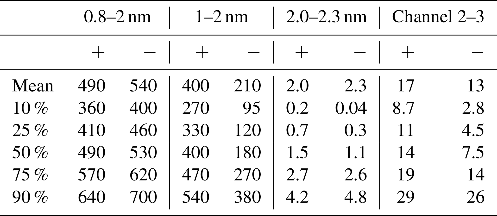
In order to find out how reliably the CIC is able to observe ion concentrations, we compared it with the NAIS at the SMEAR II station in Hyytiälä, Finland. Tables 1 and 2 summarize the percentiles of the ion concentrations measured by these two instruments for different size fractions. We can see that the total concentration of sub-2 nm negative ions measured by the NAIS is significantly higher than that measured by the CIC (channel 1), the median concentrations being equal to 530 and 210 cm⁻³, respectively. This result is expected, as the detection efficiency of both instruments decreases rapidly for particles smaller than 1 nm. However, the NAIS is able to correct for this in data inversion, while the CIC is not due to the lack of detailed information about the measured size distribution. Excluding the smallest ions measured by the NAIS, i.e., considering only the 1–2 nm size range, the median concentration drops down to 180 cm⁻³. This is slightly below the median sub-2 nm concentration measured by the CIC but only about one-third of the median total sub-2 nm ion concentration measured by the NAIS.

Table 1 Percentiles of the CIC channel 1 (small ion) and channel 2–3 (roughly 2.0–2.3 nm ion) concentrations (cm⁻³) during 16 January–1 April 2024. Positive polarity is marked by + and negative by −. The negative concentrations for the channel 2 subtracted by channel 3 are indicative of a noisy signal of the instrument.

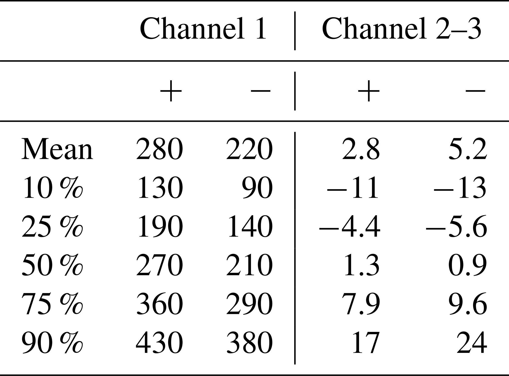
Table 2 Percentiles of NAIS concentrations (cm⁻³) during 16 January–1 April 2024, excluding 16–17 March 2024. Small ions in the diameter ranges 0.8–2 nm and 1–2 nm are included. Intermediate ion concentrations are included for diameter range 2.0–2.3 nm, as well as for the diameter range that the CIC covers (channel 2–3; see Sect. 2.3 for details). Positive polarity is marked by + and negative by −.

A comparison between the two instruments is in Fig. 2 for small (1–2 nm) ions and in Fig. 3 for the smallest size class of intermediate ions (2.0–2.3 nm). We can see that when the small ion concentration is above 200 cm⁻³, the two instruments show similar values, while at lower concentrations there is more spread in the values, with the CIC generally measuring higher concentrations than the NAIS. At low concentrations, it is possible that the uncertainties in the detection efficiencies of the ions with diameters close to 1 nm impact the results, explaining our observations. CIC channel 2–3 concentrations are consistently lower than NAIS channel 2–3 concentrations, with the difference being smaller when the concentrations are higher, suggesting that at lower concentrations, electronic noise increasingly impacts the comparison. There is more spread between the values of NAIS 2.0–2.3 nm and CIC channel 2–3. At higher concentrations, the CIC shows higher concentrations than NAIS 2.0–2.3 nm concentration. However, the overall agreement between these two instruments is good, with correlation coefficients of 0.85 and 0.86 for small ions and 2.0–2.3 nm ions, respectively.

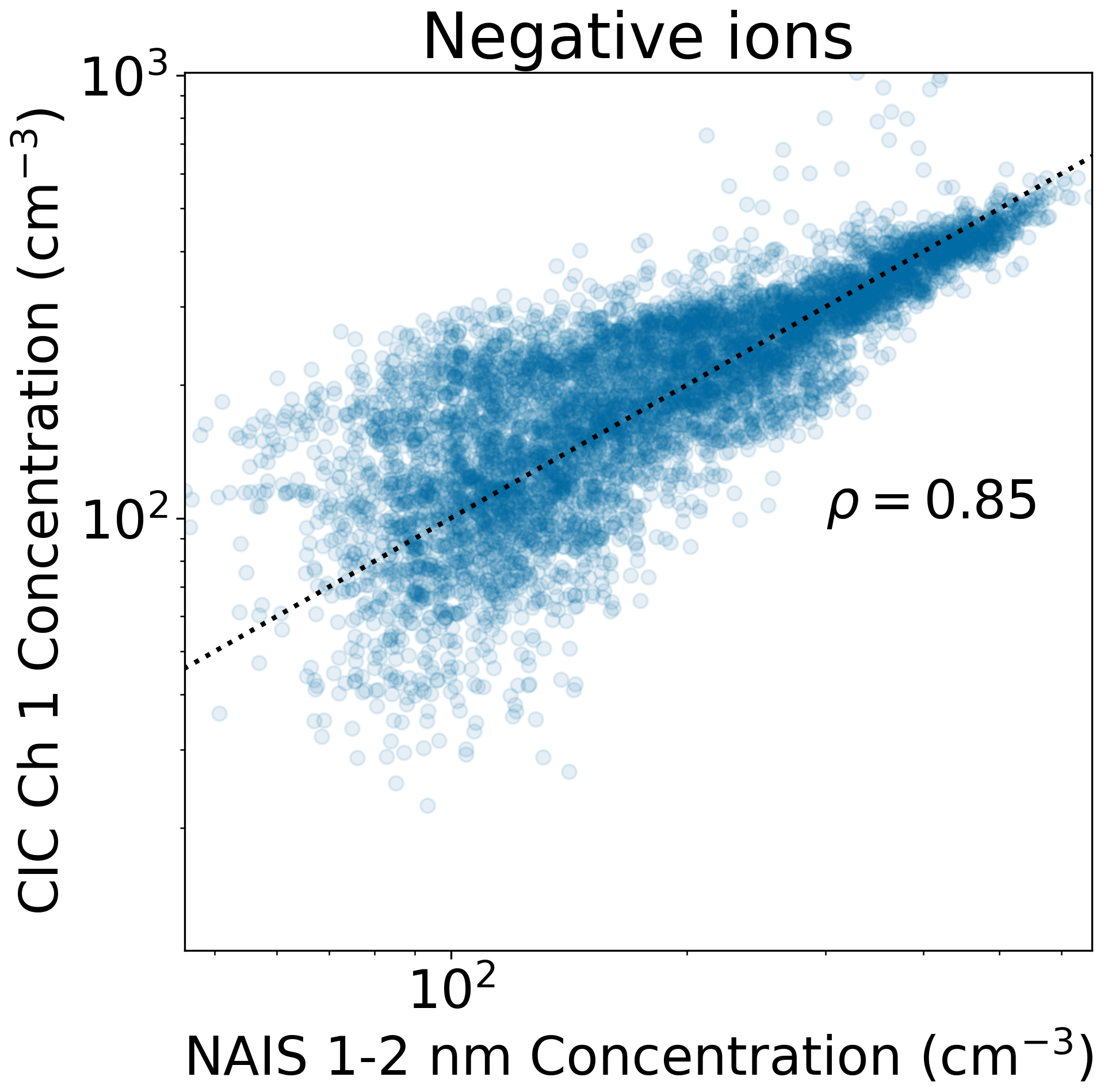
Figure 2 Scatter plot of the 15 min median negative small ion concentration measured with the CIC as a function of the concentration measured with the NAIS in Hyytiälä. The NAIS concentrations are from the diameter range 1–2 nm, while the CIC concentrations are from channel 1. The dotted black line marks the 1 : 1 line. The Pearson correlation coefficient ρ of the two concentrations shown is included in the figure.

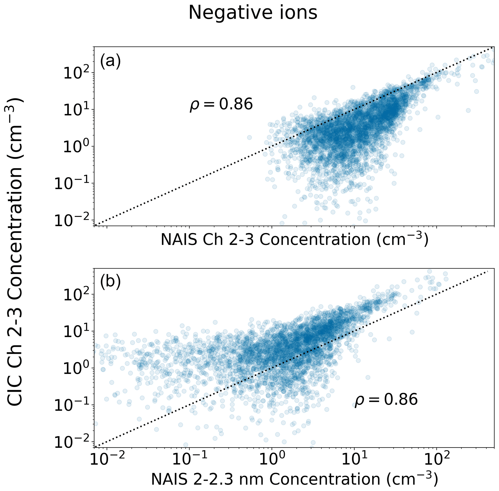
Figure 3 Scatter plot of approximately 2.0–2.3 nm negative ion 15 min median concentrations measured with the CIC as a function of concentrations measured with the NAIS in Hyytiälä. The NAIS concentrations in (a) were determined for the same size range as covered by the CIC channels 2 and 3 (for details, see Sect. 2.3). The NAIS concentrations in (b) are for the diameter range 2.0–2.3 nm. The dotted black line marks the 1 : 1 line. The Pearson correlation coefficient ρ of the two concentrations shown is included in the figure.

Figure 4 presents the time series of ion concentrations measured by the CIC and NAIS over the whole 2.5-month period, while Fig. 5 presents the diurnal pattern of ion concentrations on a selected day (10 March 2024). Total sub-2 nm ion concentrations measured by the NAIS are higher than CIC channel 1 ion concentrations. However, for the majority of the time (see Fig. 4), the NAIS 1–2 nm ion concentration and CIC channel 1 concentration are close to each other. On the selected day, CIC channel 2–3 and NAIS channel 2–3 peak values are similar, 60 and 80 cm⁻³, respectively, whereas the NAIS 2.0–2.3 nm peak value is lower at around 20 cm⁻³. CIC channel 2–3 is likely influenced by ions larger than 2.3 nm, impacting the measured concentration when intermediate ion concentration is high, such as during NPF. The correlation coefficient between the concentrations from the two instruments on the selected day is around 0.9 for both sub-2 nm and 2.0–2.3 nm ions.

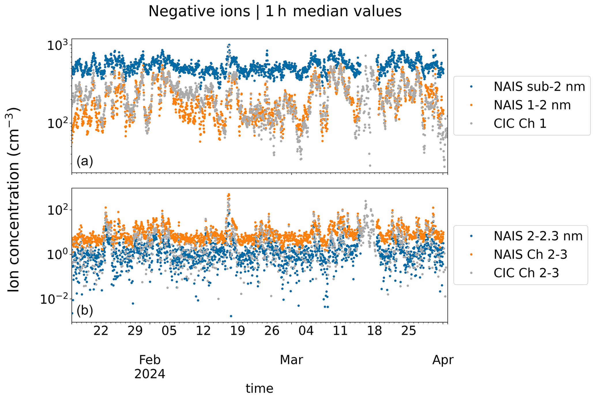
Figure 4 Time series of observed ion concentrations. Panel (a) has the concentrations of small ions from the CIC channel 1 and from the NAIS for both all sub-2 nm ions and 1–2 nm ions. Panel (b) has concentrations of ions measured by the CIC channel 2–3, which approximately corresponds to the size range of 2.0–2.3 nm. In addition, there are concentrations of 2.0–2.3 nm ions measured by the NAIS (NAIS 2.0–2.3 nm) and concentrations from the NAIS that were determined for the exact same size range as that covered by the difference of CIC channels 2 and 3 (NAIS channel 2–3).

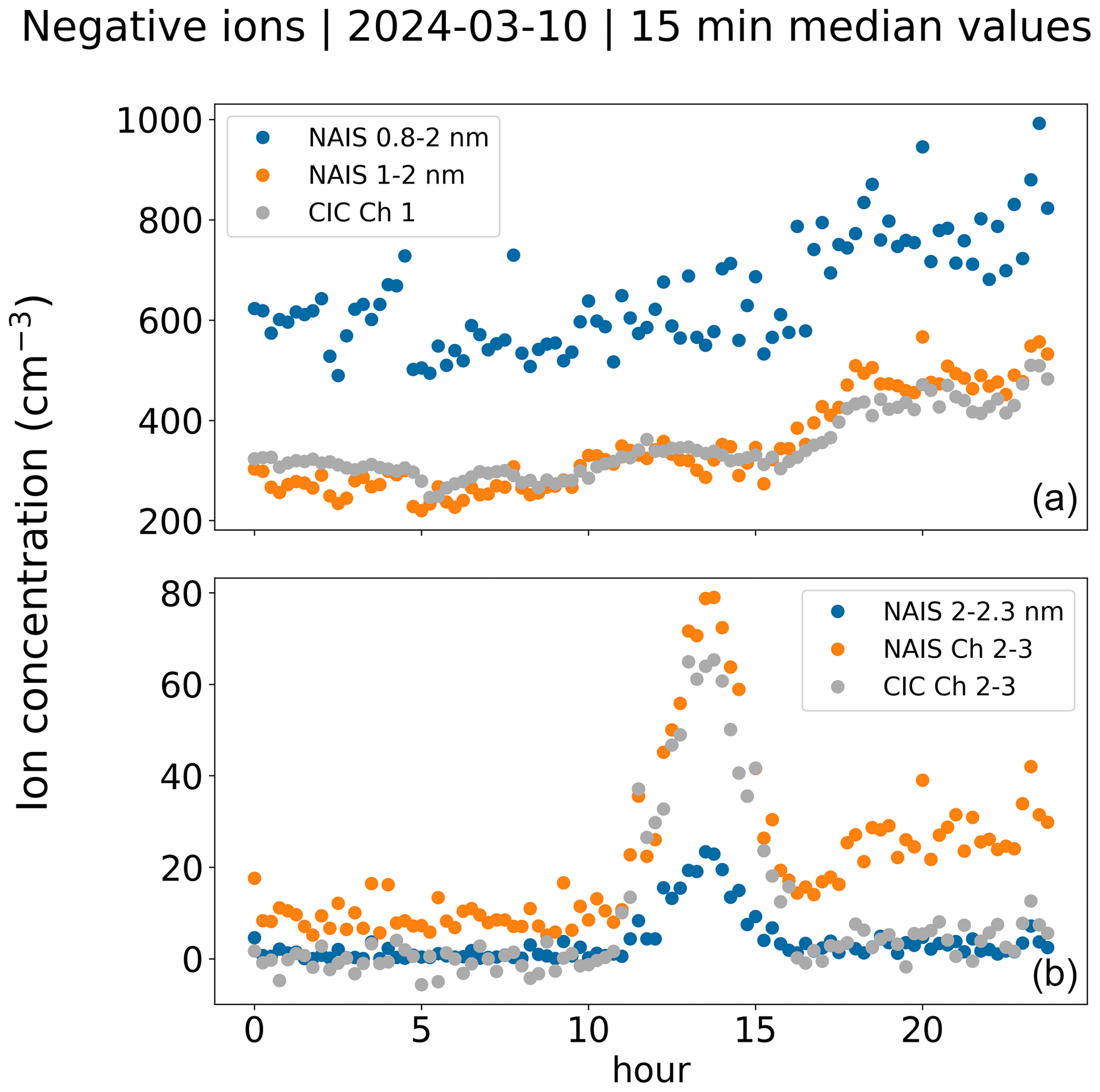
Figure 5 Observed negative ion concentrations on 10 March 2024. Panel (a) has the concentrations of small ions. For the CIC, they are from channel 1. From the NAIS, concentrations for all measured sub-2 nm ions and those based on the size range 1–2 nm are included. Panel (b) has the concentrations of intermediate ions. For the CIC, they are from channel 2–3, corresponding to roughly the 2.0–2.3 nm size range. For NAIS, the concentrations of ions between 2.0 and 2.3 nm are included, as well as the concentrations that were determined for the exact same size range as that covered by the CIC channels 2 and 3 (NAIS channel 2–3). The correlation coefficients on this day are 0.83, 0.95, 0.93 and 0.90 for NAIS 0.8–2 nm vs. CIC channel 1, NAIS 1–2 nm vs. CIC channel 1, NAIS 2.0–2.3 vs. CIC channel 2–3 and NAIS channel 2–3 vs. CIC channel 2–3, respectively.

Comparing the lower percentiles in Tables 1 and 2, it is apparent that a large fraction of CIC channel 2–3 concentrations are negative. At very low concentrations (< 1 cm⁻³), the signal is mainly noise. In addition, Figs. 4 and 5 show that the low background concentrations measured by CIC channel 2–3 are on average less than 10 % of NAIS channel 2–3 concentrations, which we postulate is due to estimation errors caused by the limited size resolution of the NAIS as well as different background noise levels of the instruments. At very low concentrations, the values from either instrument can be considered unreliable. Regardless, within the scope of this study, these background concentrations are of less interest compared to the higher concentrations. Periods of LIIF can be identified based on elevated 2.0–2.3 nm ion concentrations, and these ion concentrations can then be used to derive parameters, such as the ion formation rate, to quantify the intensity of LIIF. The comparison of the two instruments done here has shown that we can use CIC measurements to identify LIIF.

3.2 Application of CIC measurement in investigating condensation sink and local NPF

Figure 6 illustrates how the estimated condensation sink (CS) based on Eq. (5b) behaves as a function of small ion concentrations, I, for different ion production rates. In the same plot, we have included the observed variability of CS as determined from the particle number size distributions and I in both Hyytiälä and Beijing. We can see that measured and theoretically calculated estimates of CS agree with each other the best when median ion production rates are between about two and four ion pairs cm⁻³ s⁻¹ in both Hyytiälä and Beijing.

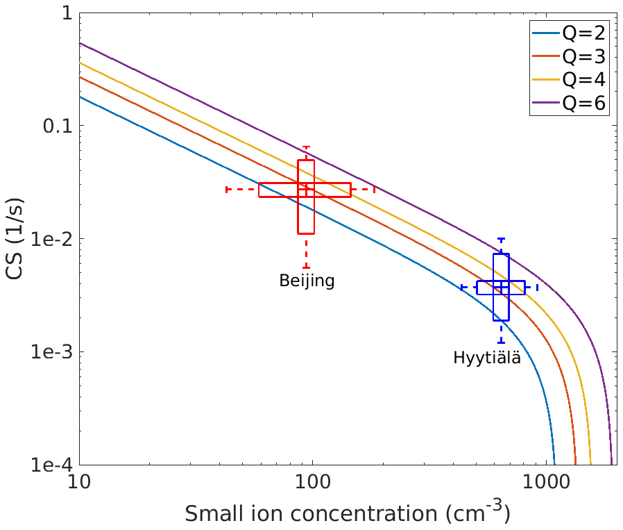
Figure 6 Condensation sink (CS) as a function of the small ion concentration for different ion source rates (Q; ions cm⁻³ s⁻¹). The observed values of I and CS in Hyytiälä and Beijing (medians marked by the center line of the box plot, 25 % and 75 % quartiles marked by the edges, and 10 % and 90 % percentiles marked by the whiskers of the box plots) indicate ion source rates between about 2 and 4 cm⁻³ s⁻¹ in both places.

The CIC has a higher detection efficiency for small ions than the NAIS due to a shorter inlet tract and, consequently, lower inlet losses. However, in the case of both instruments, the detection efficiency for sub-2 nm ions is very strongly dependent on particle size. The NAIS measures the size distribution of ions, and the data inversion algorithm uses that information to correct for the size-dependent detection efficiency. The CIC has limited information about the size distribution of detected ions, making it more difficult to correct for the detection efficiency. Using the sub-2 nm ion concentrations from the NAIS and the CIC (Tables 1 and 2), we estimated how the concentrations measured using the CIC and NAIS will influence the estimated values of CS. Using Eq. (5) and assuming the median sub-2 nm ion concentrations measured by these two instruments (Tables 1 and 2), we may calculate that the values of CS measured using the NAIS are 0.237, 0.256 and 0.266 times those measured using the CIC for Q equal to 2, 3 and 4, respectively. Therefore, if we use the CIC for estimating CS via Eq. (5a), the real CS (using NAIS and Eq. 5b) is about 0.25 times the one observed by the CIC.

Figure 7 shows the CS derived based on Eqs. (5a) and (5b) versus CS determined from the full particle number size distribution (CS_DMPS). We see that the CS predicted by NAIS varies less than CS_DMPS but is mostly within the same order of magnitude. CS predicted by the CIC is consistently higher than CS_DMPS. However, considering the above discussion, and multiplying the estimated CS by 0.25, we get values much closer to CS_DMPS. Assuming Q=2 ion pairs cm⁻³ s⁻¹, the CS values predicted by the CIC are mainly within a factor of 3 from CS_DMPS values.

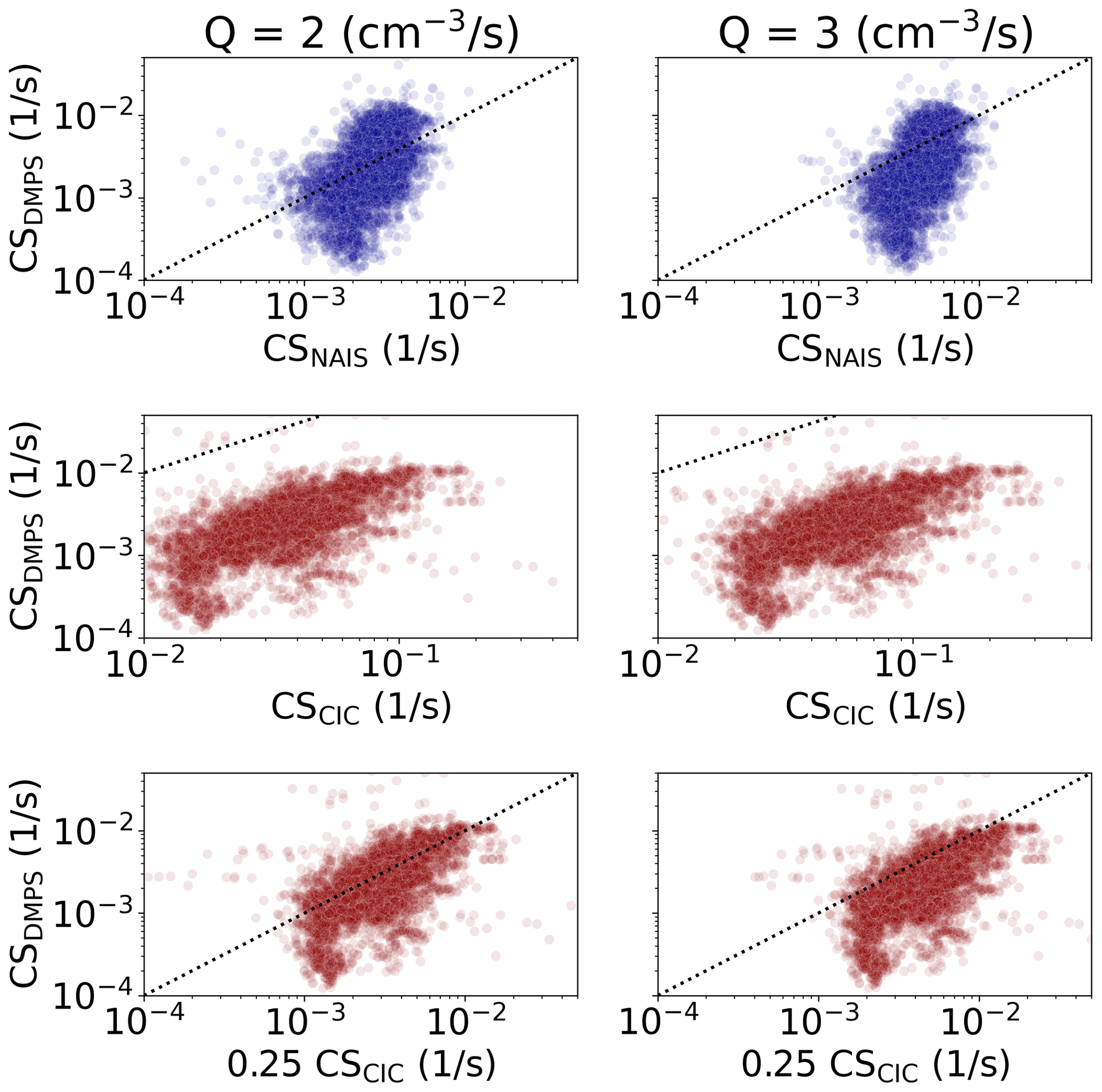
Figure 7 Condensation sink (CS) determined based on particle number size distribution data measured by DMPS versus CS derived based on negative sub-2 nm ion concentrations from the NAIS and CIC. For the CIC and NAIS, Eqs. (5a) and (5b) have been used, respectively.

We have assumed that the only losses of ions are due to their coagulation with larger particles and their recombination with oppositely charged ions. In reality, processes such as deposition also affect the ion concentration. For example, Tammet et al. (2006) found that in Hyytiälä, deposition of ions to forest canopy impacts small ion concentrations. In addition, we have assumed the ion source rate to be constant. In reality, it is expected to vary somewhat, for example, due to varying radon concentration (e.g., Hirsikko et al., 2007). Therefore, the presented method of determining CS can only give a rough approximation for CS.

In order to illustrate how the CIC can be used to determine the ion growth rate (GR), we selected one measurement day (Fig. 8) and determined the GR using the appearance time method (e.g., Lehtipalo et al., 2014) and Eq. (4). Ion concentrations from the CIC channel 2–3 and channel 3 from 13 February were used. The ion concentrations were smoothed using a moving 1 h median method to lessen the impact of noise. As we can see from Fig. 8, channel 3 and channel 2–3 concentrations on the selected day have a similar shape between 10:00 and 16:00, and the shape of the channel 3 roughly follows that of channel 2–3 with a time delay. Considering the shape and features of the two curves, and the times at which the two concentrations reach a similar fraction of the maximum concentration (appearance time method), two time instances were identified visually. The appearance times were chosen to correspond to times when the ion concentrations were around 20 % of the maximum concentrations. From these approximate appearance times, a time delay was calculated. Based on Fig. 1, the diameters of 2.2 and 2.9 nm for channel 2–3 and 3 were assumed, respectively. We note that on this particular example day, the curves follow each other closely for a span of several hours, and therefore the value of the GR is not very sensitive to the identified appearance times; i.e., the chosen fraction of the maximum concentration anywhere between 0.2 and 0.9 results in the same approximate GR. The resulting GR was approximately 0.9 nm h⁻¹. This value is in the expected range, as the earlier long-term measurements at the same site indicate typical growth rates between about 1 and 2 nm h⁻¹ for sub-3 nm ions (Hirsikko et al., 2005; Manninen et al., 2010). We should note, however, that it is not possible to determine GRs for all measurement days using the procedure presented here. This is because even if an increase in ion concentrations were observed, the signal might be too noisy, making the determination of appearance times too unreliable. In addition, not all days exhibited a clear delay between the two appearance times, making the determination of growth rate impossible.

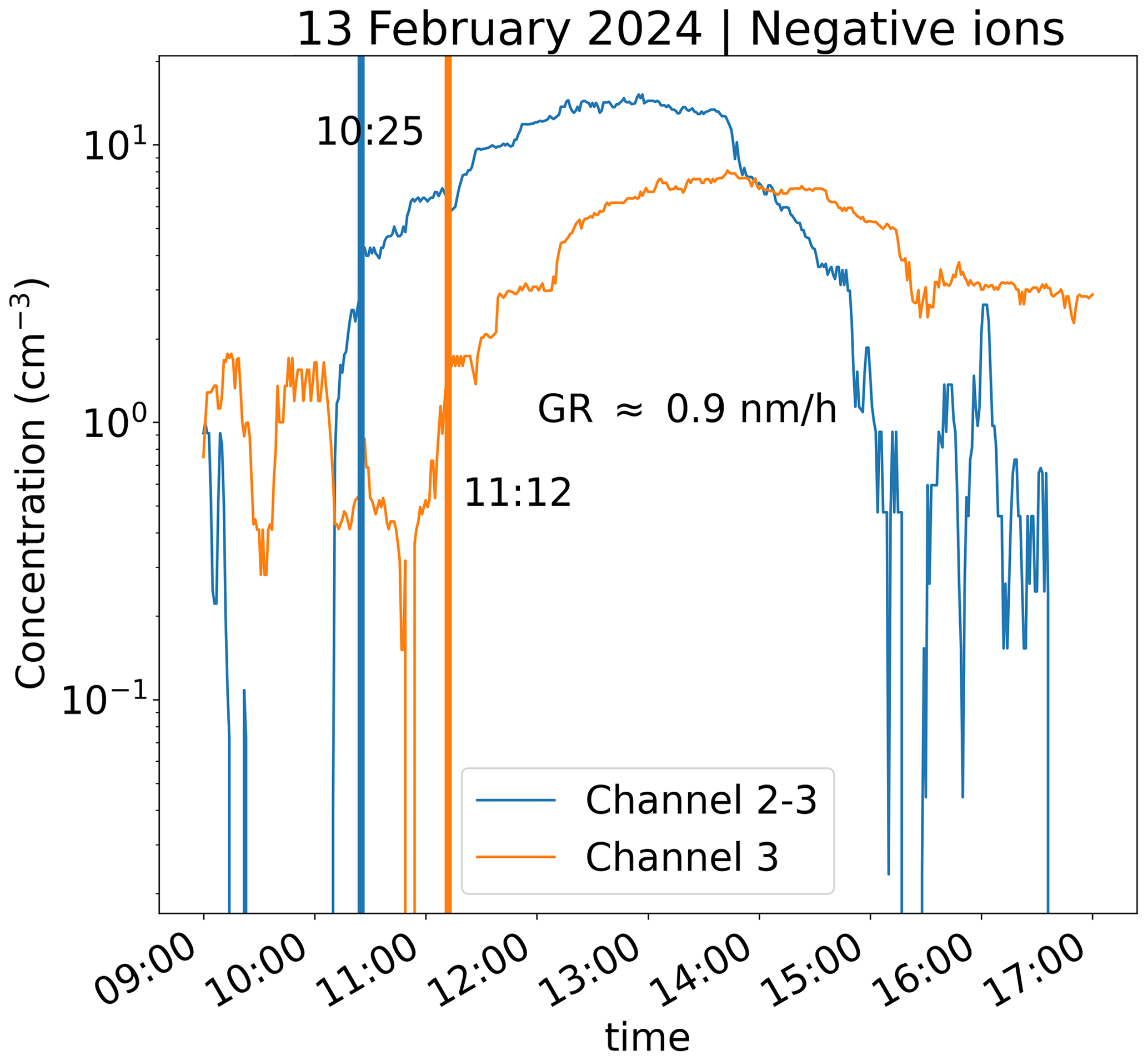
Figure 8 The CIC channel 3 and channel 2–3 concentrations on the day of 19 February. Approximate appearance times have been marked by vertical lines alongside the growth rate (GR) from 2.2 to 2.9 nm derived based on those appearance times.

Using Eq. (9), we can estimate the formation rate of 2 nm ions, J₂. Figure 8 shows these formation rates for Hyytiälä and Beijing. This formation rate can be given as a function of the measured number concentrations of 2.0–2.3 nm intermediate ions, in addition to which J₂ depends on the growth rate, ion source rate and ion loss rate, the latter of which was estimated using the sub-2 nm ion concentrations according to Eq. (5b). J₂ also depends on the concentration of sub-2 nm ions, which is determined by the ion loss rate and ion source rate (Eq. 1). For Fig. 9, the median sub-2 nm ion concentrations in Hyytiälä and in Beijing were used in Eq. (9). The most probable values are 1–2 nm h⁻¹ for the growth rate in Hyytiälä (Fig. 8; Hirsikko et al., 2005; Manninen et al., 2010), 1–3 nm h⁻¹ for the growth rate in Beijing (Deng et al., 2020) and 2–3 cm⁻³ s⁻¹ for the ion source rate (Fig. 6). However, also higher values are given for comparison. Manninen et al. (2010) calculated a median value of 0.06 cm⁻³ s⁻¹ for J₂ based on long-term measurements in Hyytiälä, which is at the higher end of values estimated in Fig. 9. Compared with Hyytiälä, we estimate values of J₂ that are a factor of 2–4 larger for Beijing. If one wants to estimate the total 2 nm particle formation rate, in both places, it is considerably larger than the formation rate of 2 nm ions, being of the order of one magnitude in Hyytiälä (Manninen et al., 2010; Kulmala et al., 2013) and even larger in Beijing (Deng et al., 2020). These results are fully consistent with the general finding that on average, observed new particle formation rates are 1 to 3 orders of magnitude larger in polluted urban environments compared with clean or moderately polluted environments (Kerminen et al., 2018; Nieminen et al., 2018), whereas the average formation rates of 2 nm ions are typically within a factor of 2–3 between different environments (Manninen et al., 2010).

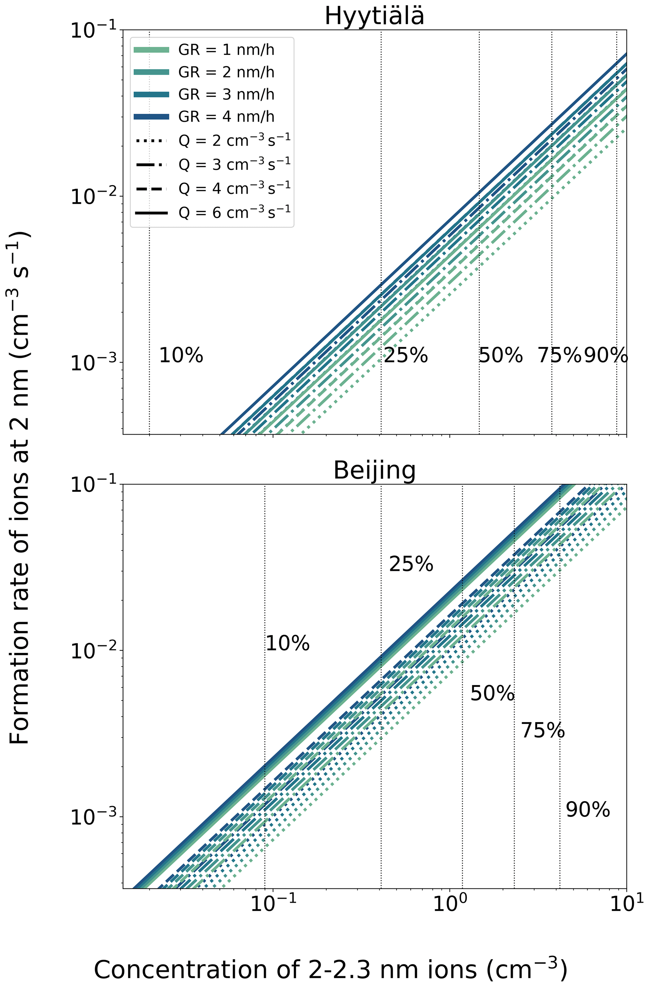
Figure 9 The estimated formation rate of 2 nm negative ions as a function of the concentration of 2.0–2.3 nm ions. The ion growth rate has been assumed to be equal to 1 nm h⁻¹. The 10 %, 25 %, 50 %, 75 % and 90 % concentration values are indicated by the vertical lines.

Figure 10 shows the estimated time evolution of the condensation sink and 2 nm ion formation rate during one day. The estimated value of CS varies only little, by less than a factor of 1.5, whereas the ion formation rate varies by more than 2 orders of magnitude during the day. We can clearly see that when the estimated CS is at its lowest at around midday, the ion formation rate is at its highest.

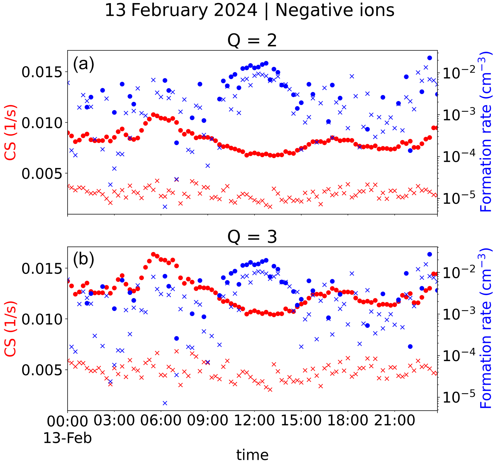
Figure 10 Condensation sink (left-hand y axis) and formation rate of 2 nm ions (right-hand y axis). The values marked by dots are based on CIC channel 1 and channel 2–3 ion negative ion concentrations, while the values marked by crosses are based on NAIS sub-2 nm and 2.0–2.3 nm negative ion concentrations. Panel (a) has values with an assumed ion source rate of Q=2 cm⁻³ s⁻¹, while panel (b) includes those for Q=3 cm⁻³ s⁻¹. A value of 0.9 nm h⁻¹ for the GR was used, as determined in Fig. 7 for this day. Negative and positive ion concentrations were assumed to be the same.

4 Conclusions and summary

The recent progress on finding local NPF (e.g., Kulmala et al., 2024b; Tuovinen et al., 2024) has opened up the following question: are we able to utilize a simple ion counter to identify and quantify LIIF in a proper way? According to our results presented above, the answer is yes.

We have developed a modified version of the CIC to measure sub-2 nm ion and 2.0–2.3 nm ion concentrations as accurately as possible (Mirme et al., 2024). From the former quantity we get information on the dynamics of small ions, including an estimate of the coagulation sink of ions and, via Eqs. (2) and (5), also condensation sink. Furthermore, the CIC makes it possible to estimate the growth rate from about 2 to 3 nm and, with this information, the formation rate of 2 nm ions, which we can use to quantify the intensity of LIIF. While we have focused on negative ions in this paper, the same principles are also valid for positive ions. LIIF is more sensitive to negative ions (Tuovinen et al., 2024), and thus negative ions were investigated.

We compared the CIC with the NAIS in Hyytiälä, which demonstrates that the measured ion concentrations from the CIC are able to capture the temporal behavior of the ions such as the variation in concentrations due to LIIF. The comparison of the estimated condensation sink from ion concentrations using the ion balance equation with the observed ones in Hyytiälä and Beijing demonstrates how the CIC, together with the simple theoretical framework, can be used to estimate condensation sink, coagulation sink of ions and the ion formation rate. In addition, the comparison of estimated CS based on CIC measurements with the CS determined particle number size distributions shows that we can get estimates that are within a factor of 3 of the real CS. Therefore, we can conclude that the CIC is an effective instrument to observe LIIF and CS. Since the CIC is ca. 7 times cheaper and requires less maintenance than NAIS, with the CIC, one can have more observation locations and have wider data coverage than with NAIS. However, if we want to investigate aerosol formation and growth rates for the nucleation mode (3–25 nm), as is usually the case in investigating regional NPF, NAIS measurements are needed.