A multi-instrumental approach for calibrating real-time mass spectrometers using high-performance liquid chromatography and positive matrix factorization

Obtaining quantitative information for molecular species present in aerosols from real-time mass spectrometers such as an extractive electrospray time-of-flight mass spectrometer (EESI) and an aerosol mass spectrometer (AMS) can be challenging. Typically, molecular species are calibrated directly through the use of pure standards. However, in some cases (e.g., secondary organic aerosol (SOA) formed from volatile organic compounds (VOCs)), direct calibrations are impossible, as many SOA species can either not be purchased as pure standards or have ambiguous molecular identities. In some cases, bulk OA sensitivities are used to estimate molecular sensitivities. This approach is not sufficient for EESI, which measures molecular components of OA, because different species can have sensitivities that vary by a factor of more than 30. Here, we introduce a method to obtain EESI calibration factors when standards are not available, and we provide a thorough analysis of the feasibility, performance, and limitations of this new technique. In this method, complex aerosol mixtures were separated with high-performance liquid chromatography (HPLC) followed by aerosol formation via atomization. The separated aerosols were then measured by an EESI and an AMS, which allowed us to obtain sensitivities for some species present in standard and SOA mixtures. Pure compounds were used to test the method and characterize its uncertainties, and obtained sensitivities were consistent within ±20 % when comparing direct calibrations vs. HPLC calibrations for a pure standard and within a factor of 2 for a standard mixture. In some cases, species were not completely resolved by chromatography, and positive matrix factorization (PMF) of AMS data enabled further separation. This method should be applicable to other real-time MS techniques. Improvements in chromatography are possible that would allow better separation in complex mixtures.

1 Introduction

Atmospheric aerosols are a complex, and often poorly understood, component of Earth's atmosphere. Aerosols have significant effects on both human and ecosystem health and are significant contributors to anthropogenic climate forcing (Dockery et al., 1996; Lighty et al., 2000; Lohmann et al., 2004; IPCC, 2013). Organic aerosol (OA) is a substantial component of global aerosol levels (Kanakidou et al., 2005; Zhang et al., 2007; Jimenez et al., 2009). Since the early 2000s an important instrument for measuring OA concentrations in real time has been the aerosol mass spectrometer (AMS) (Jayne et al., 2000; Canagaratna et al., 2007) and its high-resolution version (HR-AMS) (DeCarlo et al., 2006). Soft ionization aerosol mass spectrometers, such as the extractive electrospray time-of-flight mass spectrometer (EESI ToF MS, EESI hereinafter), have more recently become important tools for obtaining more detailed OA speciation (Lopez-Hilfiker et al., 2014, 2019; Eichler et al., 2015).

EESI can detect individual molecular ions (referred to henceforth as either molecular ions or individual species, even if they may comprise several isomers) from the particle phase with 1 s time resolution (Lopez-Hilfiker et al., 2019; Pagonis et al., 2021). EESI has been used to measure aerosols in urban areas (Qi et al., 2019, 2020; Stefenelli et al., 2019; Kumar et al., 2022), in biomass burning (Qi et al., 2019; Pagonis et al., 2021), in cooking emissions (Qi et al., 2019; Brown et al., 2021), and for chamber studies of secondary OA (SOA) formation (Liu et al., 2019; Pospisilova et al., 2020). Many studies have illustrated the low detection limits, limited fragmentation, and other capabilities of the EESI (e.g., Lopez-Hilfiker et al., 2019, and Pagonis et al., 2021).

However, obtaining quantitative information for individual species from EESI measurements of complex mixtures of unknown species can be challenging. This is due to each species having different and often hard to predict sensitivities (Law et al., 2010; Lopez-Hilfiker et al., 2019; Brown et al., 2021; Wang et al., 2021). In addition, EESI measures molecular ions but can in some cases cause fragmentation, such as due to loss of HNO₃ from nitrates (Liu et al., 2019). For SOA from a single precursor, the bulk sensitivity compared to SOA formed from a different precursor has been shown to vary by a factor of 15 or more (Lopez-Hilfiker et al., 2019). Different studies also show that the bulk sensitivity for OA formed from different emission sources (e.g., cooking, biomass burning,) can vary by a factor of ∼ 10 (Qi et al., 2019; Stefenelli et al., 2019; Brown et al., 2021). For pure organic standards, the sensitivity can vary by a factor of 30 or more (Lopez-Hilfiker et al., 2019). Instead of directly measuring compound sensitivity, some groups use machine learning (Liigand et al., 2020) or thermodynamic modeling (Kruve et al., 2014) to approximate instrument response factors for individual species. Other studies use bulk calibration factors for complex mixtures as an approximation for quantification (Tong et al., 2022).

Sensitivities can vary due to differences in analyte solubility (Law et al., 2010), EESI working fluid composition, sample composition, and different instrument conditions and settings, including polarity and changes in inlet pressure (Lopez-Hilfiker et al., 2019; Pagonis et al., 2021). Calibrating the EESI for individual species can be a challenging task, especially when standards are unavailable for most atmospheric oxidation products. In addition, OA from chamber experiments or field studies often contains unidentified molecular ions or those whose species identity is ambiguous.

Several calibration methods have been applied to EESI. For example, direct calibrations were performed for many organic standards in Lopez-Hilfiker et al. (2019), for 4-nitrocatechol (EESI−) and levoglucosan (EESI+) in Pagonis et al. (2021) to track sensitivity during each aircraft flight, and levoglucosan for regular sensitivity tracking during an indoor cooking study (and several other compounds less frequently and bracketing the campaign) in Brown et al. (2021). During research field studies, often only one or two species are calibrated frequently, and the rest are quantified using relative response factors measured less frequently (Qi et al., 2019; Brown et al., 2021; Pagonis et al., 2021).

A recent study combined measurements from the Vocus Proton Transfer Mass Spectrometer (Vocus), AMS, and EESI to measure speciated response factors without the need for standards. In that study, SOA was generated using an oxidation flow reactor (OFR). Following SOA formation, the Vocus measured the gas phase species, and the AMS and EESI measured the bulk and speciated particulate phase, respectively. EESI response factors were obtained through comparison to decreasing gas phase mixing ratios measured by the Vocus as they condensed to the particle phase (Wang et al., 2021).

Another method for obtaining calibration information is positive matrix factorization (PMF). PMF is a type of factor analysis that allows approximate apportioning of aerosol mass measured with online mass spectrometers and other instruments to atmospheric sources or level of oxidation (Zhang et al., 2005; Lanz et al., 2007; Ulbrich et al., 2009). To our knowledge, PMF has not been used with AMS data alone to obtain mass spectra and time series for individual molecular components. Separation with PMF alone could be difficult for ambient or chamber experiment data since most compounds likely covary in time and thus would not be statistically resolvable (Craven et al., 2012). Direct calibrations have been conducted to generate high-resolution AMS mass spectra for individual species (Ulbrich et al., 2019). A combination of AMS and PMF has been used to obtain quantitative information for EESI bulk measurements or PMF factors (Qi et al., 2019, 2020; Kumar et al., 2022). PMF has also been used on a combined data set consisting of both EESI and AMS data (Tong et al., 2022).

To our knowledge, PMF has not been applied previously to AMS and EESI chromatographically separated data. Running PMF on chromatographic data may be able to generate species-specific mass spectra and time series for compounds that cannot be obtained as pure standards. PMF has been applied in the past to gas chromatography mass spectrometry (GC MS) data (Zhang et al., 2014, 2016; Gao et al., 2018), but not to high-performance liquid chromatography (HPLC) data, which is better suited for oxidized SOA species than GC, to our knowledge. AMS detection following HPLC separation has been conducted previously (Farmer et al., 2010) to explore AMS spectra of the separate compounds, but not for quantification. HPLC has not been previously combined with EESI or PMF, to our knowledge. Further, HPLC must be used here because the mass spectrometric detection needs to be much faster than the chromatographic timescale (on the order of seconds). Otherwise, this method is not applicable, and the different species separated by the chromatography would not be sufficiently resolved for speciated detection with the EESI and AMS.

Here, for the first time, we demonstrate a method combining HPLC, atomization, and detection by EESI, AMS, and scanning mobility particle sizer (SMPS). The method was validated by running pure standards, standard mixtures, and chamber SOA. The analyte peaks measured with each instrument were integrated, and calibration factors for separated species were calculated for the EESI (${\mathrm{CF}}_x^{\mathrm{E}}$). The AMS response factor (${\mathrm{CF}}_x^{\mathrm{A}}$, or relative ionization efficiency (RIE) collection efficiency (CE), the product of the relative ionization efficiency and collection efficiency) and the atomic oxygen-to-carbon (O : C) ratio for different analytes were quantified. EESI calibration factors (${\mathrm{CF}}_x^{\mathrm{E}}$) for individual compounds were determined and compared to literature values. In cases where HPLC did not fully resolve all analytes, PMF was run on the AMS mass spectral matrices to obtain further compound separation.

2 Methods

2.1 Chamber experiments and filter mass collection

SOA was generated using the procedure of DeVault et al. (2022). Briefly, chamber experiments were conducted in an 8.0 m³ Teflon chamber (Claflin and Ziemann, 2018; Bakker-Arkema and Ziemann, 2021). The temperature (23 °C) and atmospheric pressure (0.83 atm) were constant. Ammonium sulfate seed was added to the humidified chamber (RH = 55 %), followed by β-pinene, which was evaporated from a heated glass bulb. In the dark, N₂O₅ was added as the NO₃ source, from the sublimation of cryogenically trapped solid N₂O₅. During these experiments, ∼ 372–1378 µg m⁻³ SOA was made within the large reaction chamber. This material was collected on a filter for ∼ 120 min at a flow rate of 14 L min⁻¹. Following dissolution in solvent, ∼ 16–56 µg of SOA was injected into the HPLC. Further discussion is included in Sect. S4 in the Supplement. The experiment was modeled after Claflin et al. (2018).

Following SOA formation, a 0.45 µm Millipore Fluoropore PTFE filter was used to collect SOA. The combined filter and aerosol was weighed after aerosol collection. The combined filter and aerosol was exposed to minimal ambient air and was always handled with artificial lighting turned off and outdoor blinds drawn. After weighing, each filter was extracted in 2 mL of HPLC grade ethyl acetate (EtAc) twice. The 4 mL aerosol extract / EtAc mixture was dried using pure N₂. Once the EtAc was evaporated, the leftover material was dissolved in HPLC grade acetonitrile (ACN) and stored in a freezer at −23 °C (DeVault et al., 2022). The extract used here was the same as DeVault et al. (2022) and was 1 year old at the time of analysis. DeVault et al. (2022) showed that this SOA is composed entirely of acetal dimers, which are exceptionally stable. Therefore, the SOA is unlikely to have changed significantly over this period.

2.2 High-performance liquid chromatography (HPLC)

HPLC separation was performed using a Shimadzu Prominence HPLC, coupled to a Zorbax Eclipse XDB-C18 column (250 × 4.6 mm with 5 µm particle size). A Nexera X2 SPDM30A UV–Vis photodiode array detector was used to generate absorbance chromatograms. The column stationary phase was designed for reverse mode, where smaller, more polar species had shorter elution times. Separated species were measured first at λ = 210 nm and λ = 254 nm using a UV–Vis diode array detector with a reference wavelength of 300 nm. Separated chemical components then flowed into a high-flow Collison atomizer, forming droplets and then aerosols consisting solely of the SOA compounds after evaporating the HPLC solvent in a Nafion dryer. The aerosols were then measured by a suite of instruments, shown in Fig. 1 and pictured in Fig. S1. Tubing delay times are also included in Table S1.

Figure 1 HPLC schematic. Left: HPLC containing a column and a UV–Vis detector. Following separation, the column effluent was sent to an atomizer and dried, and the aerosol was detected by each of the instruments shown.

A maximum volume of 50 µL ACN $/$ aerosol mixture was injected into the column at once. At the beginning of each day, the HPLC solvent lines (HPLC grade acetonitrile and HPLC grade water) were flushed to remove any air bubbles that may affect elution. Following this, a clean cycle was run by injecting 50 µL HPLC grade ACN into the reverse phase column. This ensured previous HPLC run species did not contaminate new runs. The first run of the day, post-cleaning cycle, was a 4-nitrocatechol $/$ 4-nitrophenol mixture (dissolved in ACN). These species were well characterized by the particle phase instruments and have measurable absorbances at the recorded UV wavelengths.

For each experiment, the mobile phase consisted either of an ACN $/$ water mixture or an ACN $/$ CH₃OH $/$ water mixture. The mixture varied in relative concentrations of each solvent over the course of each HPLC run. Most experiments were started at 95 % water / 5 % ACN (solvent mixture A). The mobile phase became less polar over time. For some systems, solvent B (pure acetonitrile) replaced solvent system A as time went on. For other systems, solvent C (pure methanol) was used. Each standard and/or SOA system was run under different conditions, depending on the separability of different components.

For the standard solution run, a mixture of solvent A and solvent B was used. Using a flow of 1.0 mL min⁻¹, solvent B was increased from 0 % to 35 % in 1 min, then 35 %–40 % for 5 min, followed by 40 %–50 % for 3 min, and 50 %–100 % for 2 min. This is also shown in Fig. S2a. For the β-pinene SOA extract, the flow rate was set to 0.5 mL min⁻¹, and a mobile phase gradient started at 20 % solvent C for 2 min, then increased at a rate of 6 % min⁻¹ up to solvent C of 50 %, followed by an increase of 3 % min⁻¹ to a concentration of 80 % solvent C, then 0.75 % min⁻¹ until 95 % solvent C, held at 95 % C for 20 min, and increased by 1.7 % min⁻¹ to 100 %, following 10 min at 100 % solvent B, shown in Fig. S2b (DeVault et al., 2022).

2.3 Standards for HPLC measurements

Two standard solutions of atmospherically relevant species were made for this study. Standard solution 1 contained 0.4 % (by mass) 3-methyl-4-nitrophenol, 0.2 % phthalic acid, 0.5 % 4-nitrophenol, 0.6 % succinic acid, and 0.1 % 4-nitrocatechol, dissolved in HPLC grade acetonitrile. Solution 2 contained six species: 0.3 % phthalic acid (by mass), 0.3 % L-malic acid, 0.1 % succinic acid, 0.3 % citric acid, 0.3 % levoglucosan, and 0.2 % 4-nitrocatechol in HPLC grade acetonitrile. Source information and calculated saturation mass concentrations for all species are shown in Table S2.

Each species was chosen for its relevance in biomass, urban, or manufacturing processes; 3-methyl-4-nitrophenol, 4-nitrophenol, 4-nitrocatechol, and levoglucosan are cyclic C₆ carbon species found in biomass burning. Succinic acid, L-malic acid, and phthalic acid are acids of secondary origin found in urban atmospheres. Citric acid is found in food and/or medicine. A critical property of these compounds is that they absorb in the UV–Vis, whereas most SOA does not. Nitrates and aromatics have strong absorbance, and carboxylic acids have a very weak absorbance.

2.4 Aerosol generation and sampling system

The HPLC was coupled to particle phase measurements by using a high-flow Collison atomizer. First, a Teflon line was attached to the waste port of the HPLC. The flow from the HPLC was 0.5–1 mL min⁻¹, all of which was sent to the atomizer. The atomizer operated by first introducing pressurized compressed air (∼ 20 psi) into a small chamber (473 mL jar). Perpendicular, sample flow at a rate of 0.5 or 1 mL min⁻¹ intersected the pressurized air. This led to the generation of particles of a consistent size distribution and provided a total flow ranging from 8 to 10 L min⁻¹. Instrument-specific flows were measured daily.

Following atomization, ∼ 10 L min⁻¹ of aerosol/solvent flow was sent through a Nafion dryer before being sent through an activated carbon denuder. This denuder is in a stainless-steel, ∼ 1 in. diameter and 8 in. length tube, composed of activated carbon honeycomb cross sections. Flow was then sent into each particle instrument. Solvent was efficiently removed (> 99.0 %; Pagonis et al., 2021) using the carbon denuder. Acetonitrile (a solvent used in the HPLC system) was monitored using the EESI. Denuder regeneration was typically only necessary after the first 4 h of each experiment.

Residence times in different parts of the system were estimated to enable synchronizing the aerosol instrument observations and the measured UV–Vis absorbances. Calculations shown in Table S1 suggest that a delay of at least 40 s should be observed between the UV–Vis measurement and detection with the aerosol instruments, which is consistent with the measured delay. Retention times for EESI, AMS, and SMPS may differ from each other by 1–2 s, depending on the residence times in the tubing. In addition, bypass flows (shown in Fig. 1) were added to the EESI and AMS to reduce residence times in the tubing and thus particle losses or evaporation. These delay differences were handled by shifting instrument data by the delay times.

2.5 Description of particle measurements

2.5.1 Extractive electrospray time-of-flight mass spectrometry (EESI)

EESI uses a soft ionization technique that detects particle phase analytes based on their solubility and proton affinity/adduct formation stability (Lopez-Hilfiker et al., 2019). Briefly, particle/gas sample flow was sent into the EESI source at ∼ 0.5–1 L min⁻¹, where gases are removed using a charcoal denuder (> 99 % removal efficiency for acetic acid, when regenerated daily) (Tennison, 1998; Pagonis et al., 2021). The aerosol inlet for the instrument used in this study was pressure controlled (Pagonis et al., 2021) and was run at 575 mbar. While designed for aircraft applications, the pressure-controlled inlet provides better spray and signal stability as it shields the spray from small pressure perturbations from changes in upstream inlet flow conditions. This includes perturbations caused by switching between different sampling modes and plumbing pathways. Here, the working fluid consisted of a mixture of 25 % Milli-Q water and 75 % (by volume) HPLC grade methanol. The EESI was run in two polarity modes. The positive-polarity mode (henceforth “EESI+”) contained 200 ppm of sodium iodide (NaI) (Pagonis et al., 2021). This working fluid generally forms Analyte Na⁺ adducts. The negative-polarity mode (EESI−) was doped with 0.1 % (by volume) formic acid (Chen et al., 2006; Gallimore and Kalberer, 2013; Pagonis et al., 2021). Species with a lower proton affinity than formate donate a proton and become negatively charged. This ionization mode is generally sensitive to acidic species that can readily donate a proton and become anionic.

For both polarities, a fused silica capillary (TSP Standard FS tubing, 50 µm ID, 363 µm OD) was used to transport working fluid solution from a pressurized (250–300 mbar above ambient) fluid bottle. Typical resolution at $m/z$ 150 was 4000, and mass spectra were saved every second.

The mass concentration of a species (µg m⁻³) can be quantified from its EESI signal (I_x ion counts s⁻¹) as (Lopez-Hilfiker et al., 2019)

$$\begin{array}{}\text{(1)}& {\mathrm{Mass}}_x=I_x\left({\displaystyle \frac{{\mathrm{MW}}_x}{{\mathrm{RF}}_x}}\right)\cdot {\displaystyle \frac{\mathrm{1}}{F}}.\end{array}$$

MW_x is the molecular weight of species x, F is the flow rate (in L min⁻¹), and RF_x is the combined response factor. There are fundamental parameters for EESI signal which are described further in Lopez-Hilfiker et al. (2019). Here, we define a new variable, EESI calibration factor (${\mathrm{CF}}_x^{\mathrm{E}}$, in µg m⁻³ counts⁻¹ s), such that

$$\begin{array}{}\text{(2)}& {\mathrm{Mass}}_x=I_x\cdot {\mathrm{CF}}_x^{\mathrm{E}}.\end{array}$$

Generally, ${\mathrm{CF}}_x^{\mathrm{E}}$ is directly determined by direct calibrations with standards, when possible. Here, ${\mathrm{CF}}_x^{\mathrm{E}}$ was determined by either direct calibrations using either commercially available standards or HPLC-separated analytes. Calibration factors are reported as absolute values (in units of counts s⁻¹ µg⁻¹ m³) and also relative to 4-nitrocatechol for EESI− and levoglucosan for EESI+ (unitless).

2.5.2 High-resolution aerosol mass spectrometer (HR AMS)

A high-resolution time of flight aerosol mass spectrometer (hereinafter AMS) (DeCarlo et al., 2006; Canagaratna et al., 2007) was used to obtain 1 Hz chemical composition for organic aerosol (OA) and nitrate aerosol (pNO₃). The AMS was run with an inlet flow of 0.1 L min⁻¹ and a bypass flow of ∼ 1.4 L min⁻¹. The AMS was run exclusively in “fast mode” (Kimmel et al., 2011; Nault et al., 2018), and size distributions were not recorded. AMS backgrounds were measured for 6 s every 52 s. Outside of HPLC runs, the AMS background was < 0.1 µg m⁻³. Between eluting peaks additional backgrounds were taken to test for solvent residue and/or residual influence from previous HPLC runs. These backgrounds were generally < 2 µg m⁻³ for both the AMS and the SMPSs. The detection limit (DL) and limit of quantification between eluting peaks were 0.7 and 2.2 µg m⁻³, respectively, suggesting that background-subtracted concentrations above 2.2 µg m⁻³ can be accurately measured. The latter were conducted by flowing the sampler air through a particle filter. AMS data were analyzed in the ToF AMS analysis software (PIKA version = 1.25F, Squirrel = 1.65F) (DeCarlo et al., 2006; Sueper, 2023) within Igor Pro 8 (Wavemetrics, Lake Oswego, OR). When AMS sensitivities were not obtained from direct measurements, the AMS OA RIE and CE were assumed to be 1.4 (OA_default; Canagaratna et al., 2007) and 1, respectively. The AMS NO₃ RIE ×​​​​​​​ CE (NO_3, default) was assumed to be 1.1 (Canagaratna et al., 2007). Data herein are reported in µg m⁻³, using Boulder pressure (P = 830 mbar) and average lab temperatures (∼ 20 °C).

Here, the quantification of different particle phase species that have been separated by HPLC (and thus are mostly in single component particles) is assessed for the AMS. This is a function of RIE_X × CE_X (a.k.a. “AMS response factor”, or ${\mathrm{CF}}_x^{\mathrm{A}}$) for a species X. Direct AMS calibration has been reported for many OA species (Slowik et al., 2004; Dzepina et al., 2007; Jimenez et al., 2016; Xu et al., 2018; Nault et al., 2023). An RIE of 1.4 is typically applied to ambient organic aerosols (Canagaratna et al., 2007), which has been shown to perform well in most outdoor intercomparisons (Jimenez et al., 2016; Guo et al., 2021). Laboratory measurements typically require specific calibrations, as RIE can be higher for some compounds and mixtures (Jimenez et al., 2016; Xu et al., 2018; Nault et al., 2023). CE can vary considerably, from CE = 0.15 to a CE = 1 (Docherty et al., 2013).

The material densities of the known standards were determined by running the AMS in PToF mode and calculating the density as $d_{\mathrm{va}}/d_{\mathrm{m}}$, where d_va is the aerodynamic vacuum diameter and d_m is the SMPS measured mobility diameter (DeCarlo et al., 2004). Calculated densities are shown in Table S2. For the unknown species present in the SOA, densities were estimated using the atomic ratio of oxygen plus nitrogen to carbon ([O + N] : C) and H : C, as demonstrated in Day et al. (2022), which builds upon the method of Kuwata et al. (2012), which did not account for nitrate content. The O : C ratio attributed to the non-nitrate OA was calculated per Canagaratna et al. (2015). The organic nitrate contribution was quantified per Day et al. (2022). All nitrate here was assumed to be from organic nitrate functional groups, as the aerosol studied here likely contained little inorganic nitrate. For the density calculation, the total nitrate was multiplied by the ratio of the molecular weights of NO₂ : NO₃ (46 $/$ 62) and converted into a molar concentration using the molecular weight of NO₂ (46 g mol⁻¹). Only the NO₂ functionality was included for the density calculation, since the nitrate oxygen bonded to the carbon is expected to typically be included as part of the standard AMS OA O : C estimation (Farmer et al., 2010). Carbon was also converted into a molar concentration using the molecular weight (12 g mol⁻¹). That organic nitrogen to organic carbon ratio was added to the standard AMS OA O : C ratio to obtain the organic nitrate-corrected (O + N) : C ratio.

For isolated peaks that contained organic nitrate, the organic nitrate (NO₃) concentration was added to the AMS OA to get the total measured AMS mass. The SMPS mass was then compared to the AMS mass calculated with the default ${\mathrm{CF}}_x^{\mathrm{A}}$, and the correct ${\mathrm{CF}}_x^{\mathrm{A}}$ was determined with Eq. (3) (further details in Sect. 2.7).

$$\begin{array}{}\text{(3)}& {\mathrm{CF}}_x^{\mathrm{A}}={\displaystyle \frac{{\mathrm{OA}}_{\mathrm{default}}+{\mathrm{NO}}_{\mathrm{3},\mathrm{default}}}{\mathrm{SMPS}\mathrm{mass}}}\end{array}$$

For HPLC peaks composed of multiple species (like in the β-pinene SOA sample), the average ${\mathrm{CF}}_x^{\mathrm{A}}$ was calculated by adding the average NO₃ contribution (∼ 5 %) to the measured AMS OA contribution (Fig. S3). This ${\mathrm{CF}}_x^{\mathrm{A}}$ was then applied to the AMS PMF organic chromatographic time series, in order to determine ${\mathrm{CF}}_x^{\mathrm{E}}$. For species not containing any nitrate, the NO_3, default was set to 0.

We note that some recent work has suggested that the sensitivity of organic nitrate functional groups may be lower than for ammonium nitrate (for which the nitrate is calibrated by default in AMS data processing). Thus, a correction of ∼ 62/46 may be more appropriate here for computing nitrate functional group mass concentrations (Takeuchi et al., 2021). However, due to the small nitrate contribution overall, such a correction was not applied.

2.5.3 Scanning mobility particle sizer (SMPS)

Two SMPSs were run with a 20 s offset during HPLC experiments (consisting of all TSI, Inc components) in order to improve the time resolution of the total particle volume measurement. For both SMPSs, a 3081 differential mobility analyzer (DMA) was run with a 3080 electrostatic classifier. Each was coupled with either a 3776 condensation particle counter (CPC) (referred to as SMPS A) or a 3775 CPC (SMPS B). Both systems were run in the CPC “high-flow” mode. Sample flow rates were nominally set to 1.5 L min⁻¹, but the actual (measured flow) was 1.43 and 1.49 L min⁻¹ for the 3776 and 3775, respectively. DMA sheath flows were set to 6.0 L min⁻¹. Data were compared to that acquired in a reference mode, with a sample flow of 0.3 L min⁻¹, a sheath flow of 3.0 L min⁻¹, and 120 s scans. Testing was done to ensure that number and volume distributions and integrated concentrations matched between the reference and fast scanning modes, shown in Fig. S4 and discussed in depth in Sect. S3. The SMPSs were also run concurrently during an HPLC run to confirm that data from both instruments matched (Fig. S5). Overall, the SMPSs in the reference and fast modes agreed within 10 %. Flows were measured every day, and delay times (from the SMPS inlet to the CPC detection, which affect sizing) were calculated when changes in plumbing were made. Further details on SMPS delays can be found in Table S3.

2.5.4 Direct calibration procedure

Direct calibration refers to the standard method of generating monodisperse aerosol from a calibrant solution with a Collison atomizer (TSI model 3076) drying with a Nafion dryer, size selecting at 275 nm with a TSI 3080 electrostatic classifier/3081 DMA, removing double charged particles with an impactor, measuring the particle concentration with a 3775 CPC, and measuring with the EESI and/or AMS. The EESI and AMS sensitivities were obtained by comparing their signals to the particle mass calculated from the known particle volume, estimated density, and CPC particle concentration.

2.6 Positive matrix factorization (PMF)

Positive matrix factorization (PMF) (Paatero and Tapper, 1994; Paatero, 1997) is a bilinear deconvolution model that relies on the assumption of mass balance with components with constant spectral profiles. Briefly, time series for signals at individual $m/z$'s are entered into a two dimensional matrix with m rows (points in time) and n columns ($m/z$'s) (Ulbrich et al., 2009; Kumar et al., 2022). PMF works to minimize the squared weighted residuals between the measured and reconstructed matrices, producing multiple potential solutions that could explain different chemical or physical sources in a given data set, along with the total residual of each solution.

The model is solved using PMF2 (Paatero, 2007) and the multilinear engine, developed by Paatero​​​​​​​ (1999), run from the PMF Evaluation Tool (“PET”) software v3.08 in Igor Pro v8 (Wavemetrics, Lake Oswego, OR).

Choosing the best PMF solution always has a subjective component, as it is usually impossible to know the “correct” number of factors that completely capture a complex data set (Ulbrich et al., 2009). Several methods can be used to assess the validity of a given solution. First, the Q value (Q), which is the total sum of the error-weighed square residuals for a data set, is used. Q_exp is the expected value of Q if all residuals are due to random errors with the estimated precision at each point. If the individual data points in a solution are fit so that the residuals are consistent with random noise, then $Q/Q_{\exp }$ ∼ 1. Note that this also requires accurate estimation of the precision (random error) in the entire data matrix. In some situations, PMF cannot explain a data set within an acceptable error. In these situations, $Q/Q_{\exp }$ ≫ 1. All solutions here have $Q/Q_{\exp }$ ≤ 1.

The second criterion for picking the best PMF solution is by exploring the time series and mass spectra for a given solution for different approximate rotations (FPEAK values) (Lee et al., 1999; Lanz et al., 2007; Ulbrich et al., 2009). Simply, PMF rotations are non-unique solutions that are represented across multiple factors. In a real-world example, a source profile (e.g., biomass burning OA), might split across multiple PMF factor's time series and/or mass spectra, despite only being from a singular source. Factor splitting can sometimes reduce residuals and mathematically may appear as a more correct solution for a particular data set. This is where the user must thoroughly assess different solutions, specifically those with $Q/Q_{\exp }$ ≤ ∼ 1.

PMF solutions chosen here are based on the above criteria and a third: the time series of the residuals. In a chromatogram, the shape of the peaks is generally known. Here, four different instruments generate unique chromatograms: UV–Vis, AMS, EESI, and the SMPSs. Thus, across those four instruments, the shape of the chromatogram was fairly well constrained. When choosing solutions here, the shape of the chromatogram was compared to the time series of the residuals. If the residuals showed significant peaks, then that was an indicator that not enough factors were used to represent the complete chromatogram and all of the factors therein.

The m×n matrix for AMS data was generated for HR ions using the PMF export option in the PIKA data analysis software. Briefly, unit mass and high-resolution AMS data were first fit as described in Sect. 2.5.2. After confirming that all ions of interest were well fit, the organic data were exported into an m×n matrix (both signal and precision matrices). Any HR ions not associated with the families C_x, CH, CHO₁, and CHO_gt1 were removed, as NO₃ was not included in the PMF input, and the included families were the only measured ions with substantial signal during the experiments included here. PMF was run from 1–20 factors. Rotations (FPEAKS) were enabled, ranging from −1.0 to 1.0, in steps of 0.2.

2.7 Calculating calibration factors for species using the multi-instrumental method

For unknown species (or known species with an unknown AMS response factor), the following method was used to obtain EESI and AMS calibration factors:

1. Calculation of composition-dependent density was done using the measured elemental composition or $d_{\mathrm{va}}/d_{\mathrm{m}}$-measured densities from AMS and SMPS data.

2. SMPS size distributions are fit with a lognormal curve, and integrated volume concentrations are obtained.

3. SMPS-integrated volume time series were multiplied by the density, to produce the reference mass concentration time series.

4. The high-time-resolution AMS OA and NO₃ time series are obtained for an assumed RIE × CE = 1.4 (OA_default) and RIE × CE = 1.1 (NO_3, default).

5. The SMPS mass concentration time series and the AMS OA + NO₃ time series, for an individual chromatographic peak, are fit with a Gaussian distribution.

6. The AMS and SMPS Gaussian distributions are integrated (µg m⁻³ s).

7. The ${\mathrm{CF}}_x^{\mathrm{A}}$ was obtained using the ratio of the integrated SMPS to the integrated AMS time series fits (Eq. 3).

8. The time series for the EESI $m/z$ was fit with a Gaussian and integrated along the retention time.

9. The integrated Gaussian for the EESI $m/z$ was divided by the integrated AMS (OA + NO₃, after AMS calibration by the SMPS) or SMPS Gaussians to obtain ${\mathrm{CF}}_x^{\mathrm{E}}$ (counts s⁻¹ m³ µg⁻¹).

In step 9, the SMPS was used as the EESI reference for calculating ${\mathrm{CF}}_x^{\mathrm{E}}$ when the analytes were resolved from chromatography alone. As discussed for the mixtures shown in Sect. 3.1, 3.2, and 3.3, we never obtained complete chromatographic separation. In cases of overlapping analytes, the SMPS used here does not have the time resolution to be used as the EESI reference. Instead, we referenced the EESI to the AMS by first calibrating the total AMS signal to the total SMPS signal for mixed peaks. We then used PMF results for the corrected AMS data and compared individual AMS PMF factors time series to EESI time series to calculate ${\mathrm{CF}}_x^{\mathrm{E}}$.

3 Results

3.1 Mass balance of the analyte in the experimental system

There was substantial plumbing between the injected sample and the instruments measuring the analyte, where losses can occur (Fig. 1, Table S1). To better understand the experimental system, the mass flux was calculated using the known, injected mass as well as the tubing diameters, lengths, and flow rates, as shown in Fig. 2.

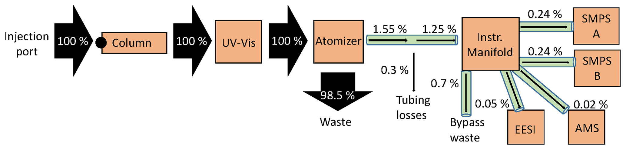
Figure 2 Mass flux across the multi-instrumental setup. Arrows are sized by the percentage of analyte mass, which is included alongside each arrow. EESI and AMS have bypass lines (represented as the total by 0.7 % bypass waste). Percentages shown are for the actual measured mass percent. Tubing details are also included in Fig. 1.

Injecting a known amount of sample into the HPLC column allowed us to track all the measured mass by the four instruments sampling. As shown in Fig. 2, all of the injected mass was analyzed by the UV–Vis spectrometer, but only a small fraction of it was analyzed (0.55 %) by the online instruments. There was substantial fluid loss at the atomizer, which is thought to account for the bulk of the mass leaving the HPLC. The EESI and AMS measure the least mass, due to their low flow rates (0.28 and 0.1 L min⁻¹, respectively). Of the mass that exited the atomizer, ∼ 20 % was lost in the tubing (∼ 10 m, ∼ $\mathrm{1}/\mathrm{4}$ in. ID) to the aerosol sampling manifold (represented as 0.3 % of total in Fig. 2). Overall, the efficiency in sampling the injected mass with the online instruments was very low with this system, primarily due to the atomization process. In SOA extracts that are highly concentrated, this is not a major problem. However, application of this method to lower-concentration samples would benefit from use of a lower-flow liquid chromatography method and a more efficient atomizer.

3.2 Application of multi-instrumental method and PMF for standard species' calibrations

3.2.1 Cross-comparison between directly calibrated one-component chromatographic standards vs. multi-instrumental method

In order to test the efficacy of the proposed method, two solutions were made containing one standard each: either phthalic acid or 4-nitrocatechol. These species were first calibrated directly in order to obtain ${\mathrm{CF}}_x^{\mathrm{E}}$ and ${\mathrm{CF}}_x^{\mathrm{A}}$, as described in Sect. 2.5.4. Then, each solution was injected into the HPLC to generate isolated chromatograms (Fig. 3).

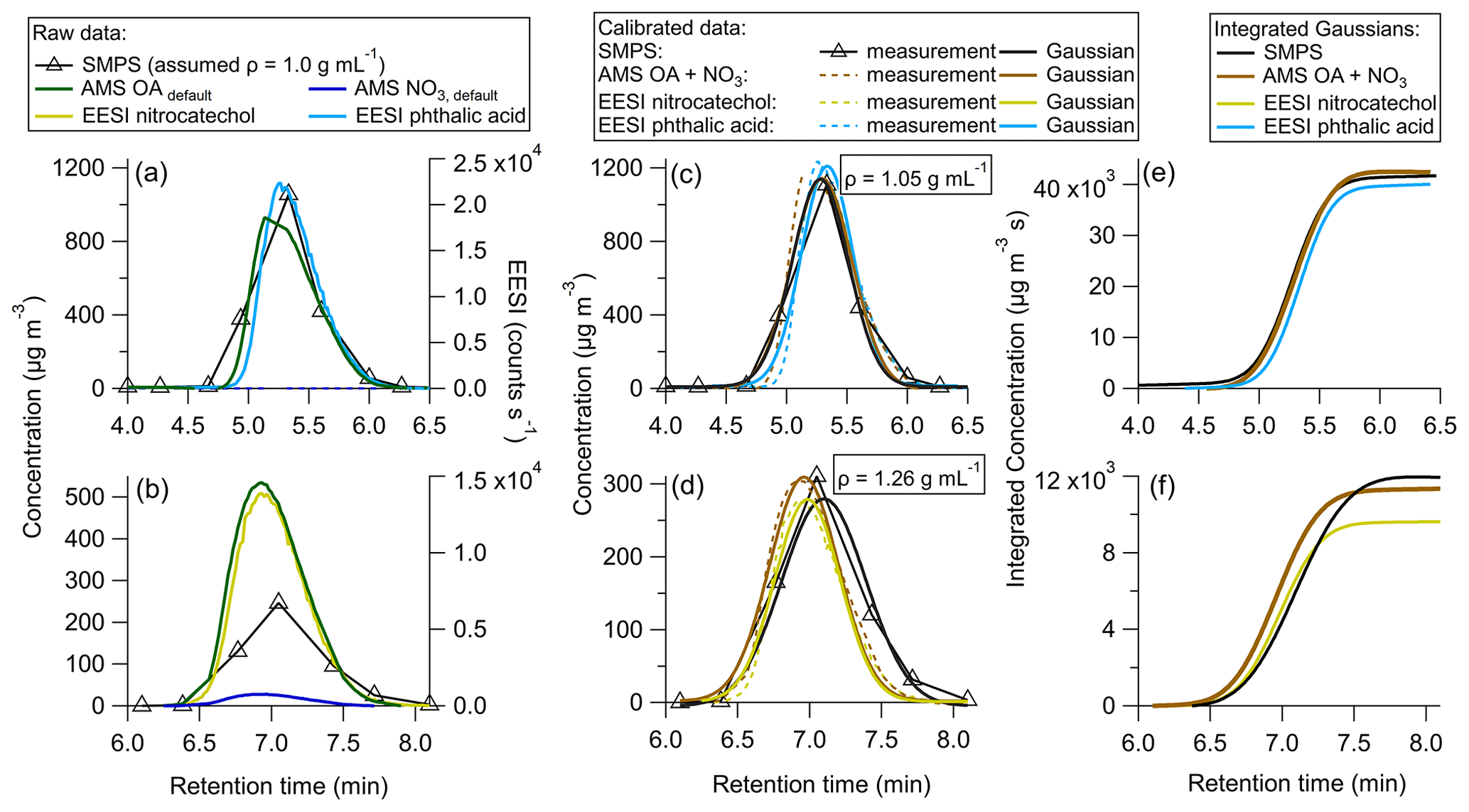
Figure 3 Single standard calibrations for (a) uncalibrated HPLC data for phthalic acid, (b) uncalibrated HPLC data for 4-nitrocatechol, (c) HPLC phthalic acid data calibrated using the sensitivity derived from the direct calibration, (d) HPLC 4-nitrocatechol data calibrated using the sensitivity derived from the direct calibration, (e) integrated Gaussian peaks from (c), and (f) integrated Gaussian peaks from (d).

In Fig. 3a, the uncalibrated background subtracted data are shown. Phthalic acid contains no nitrate moiety, so AMS NO₃ was 0. Figure 3b shows the raw data for 4-nitrocatechol. Due to the nitro group, AMS NO₃ is added to AMS OA to obtain the total mass measured by the AMS. If the method were followed as described in Sect. 2.7, the raw data would be fit with Gaussian curves and integrated, in order to produce ${\mathrm{CF}}_x^{\mathrm{E}}$ and ${\mathrm{CF}}_x^{\mathrm{A}}$ for each species. However, in this test study, ${\mathrm{CF}}_x^{\mathrm{E}}$ and ${\mathrm{CF}}_x^{\mathrm{A}}$ are already known through direct calibrations discussed in Sect. 2.5.4.

Figure 3c shows the HPLC phthalic acid peak with the direct calibration factor applied. It is clear that the AMS, EESI, and SMPS data line up well, indicating that the multi-instrumental approach produces very similar ${\mathrm{CF}}_x^{\mathrm{E}}$ and ${\mathrm{CF}}_x^{\mathrm{A}}$ as the direct calibrations. Figure 3d echoes this, showing good overlap across each instrument for 4-nitrocatechol.

Figure 3e and f show the integrated, calibrated Gaussian curves. If the multi-instrumental method worked as well as direct calibrations, the maximum integrated values would be expected to be the same for each instrument. For phthalic acid, the instruments agree within 6 %, with the EESI showing the largest deviation from the other instruments. For 4-nitrocatechol, this difference is 20 %, and again the EESI is the farthest from the other instruments. Such discrepancies could be due to changes in EESI sensitivity, which may be driven by the different solvents used for calibration (water for direct calibrations, and a mixture of acetonitrile and water for the multi-instrumental method). It could also be due to the high concentrations of each solute, which may change ${\mathrm{CF}}_x^{\mathrm{E}}$ slightly.

Figure 4 Time series of UV absorbance (milli-absorbance units) and AMS, EESI, and SMPS mass concentrations for a mixed solution standard HPLC run.

Following method validation through comparison between direct calibrations and the multi-instrumental calibration method, a mixture containing five standards (phthalic acid, 4-nitrocatechol, succinic acid, 4-nitrophenol, and 3-methyl-4-nitrophenol) was run through the HPLC column (Fig. 4). Like above, each species was first calibrated directly, in order to compare the direct calibration values vs. the multi-instrumental calibration method for a more complex chemical system.

In Fig. 4, succinic acid was the first peak to elute from the HPLC column, from ∼ 2.5–4.0 min. The EESI and SMPS data match well, but the AMS data are lower by a factor of ∼ 2. This is potentially driven by the phthalic acid–succinic acid co-elution (as evidenced by the EESI). The ${\mathrm{CF}}_x^{\mathrm{A}}$ for both species is shown in Table 1. ${\mathrm{CF}}_x^{\mathrm{A}}$ values differ substantially, and an internal mixture of aerosols containing succinic acid and phthalic acid may result in a larger AMS bias (as ${\mathrm{CF}}_{\mathrm{succinic}\mathrm{acid}}^{\mathrm{A}}$ and ${\mathrm{CF}}_{\mathrm{phthalic}\mathrm{acid}}^{\mathrm{A}}$ differ significantly) than the EESI (where we measured molecular ions) or the SMPS (as the density of phthalic acid and succinic acid are similar; Table S2).

Table 1 Calibration factors for resolved (or mostly resolved) standard species. ${\mathrm{CF}}_x^{\mathrm{E}}$ values are reported in counts s⁻¹ µg⁻¹ m³ and the relative EESI calibrations factors (${\mathrm{CF}}_x^{\mathrm{E}}/{\mathrm{CF}}_{\mathrm{nitro}}^{\mathrm{E}}$ (EESI−) or ${\mathrm{CF}}_x^{\mathrm{E}}/{\mathrm{CF}}_{\mathrm{levo}}^{\mathrm{E}}$ (EESI+)), and the AMS calibration factors (${\mathrm{CF}}_x^{\mathrm{A}}$) are unitless values.

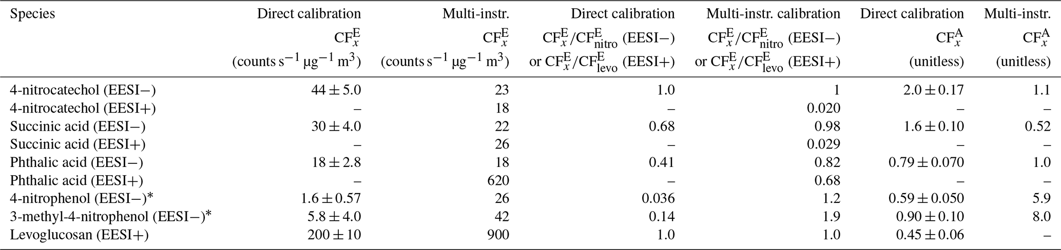
^∗ The reported values here are highly uncertain due to differences in evaporation for each instrument.

Phthalic acid elutes as two isomers, with the largest eluting between 4 and 6 min. All three instruments match well; 4-nitrocatechol was next and showed very good agreement between the EESI and AMS but a factor of ∼ 2 difference between the SMPS and EESI/AMS. The exact cause for this discrepancy is unknown.

Both 4-nitrophenol and 3-methyl-4-nitrophenol match well between the EESI/AMS, but the SMPS concentration is a factor of 20 less than the other two instruments. The likely explanation is that 4-nitrophenol and 3-methyl-4-nitrophenol are volatile (Table S2). Compared to succinic acid, > 90 % of these species evaporated from injection to detection by the EESI/AMS. The SMPS measurement is slower than the other instruments and dilutes the incoming aerosol by a factor of 4 inside the DMA column. The AMS and EESI measurements are faster and do not dilute the incoming aerosol. Due to these differences, nearly all of the injected mass evaporated in the SMPS. This suggests that volatile species (where C^∗ ≫ OA) are not able to be calibrated for by this method. Evaporation would also likely occur during direct calibrations but to a lesser degree due to the higher pure species OA concentrations.

3.2.2 Combined application of the multi-instrumental calibration method and PMF on two mixed standards solutions

PMF was combined with the multi-instrument calibration method to better separate the AMS data for succinic acid and phthalic acid, which overlap in Fig. 4. The results of applying PMF to the AMS data are shown below in Fig. 5.

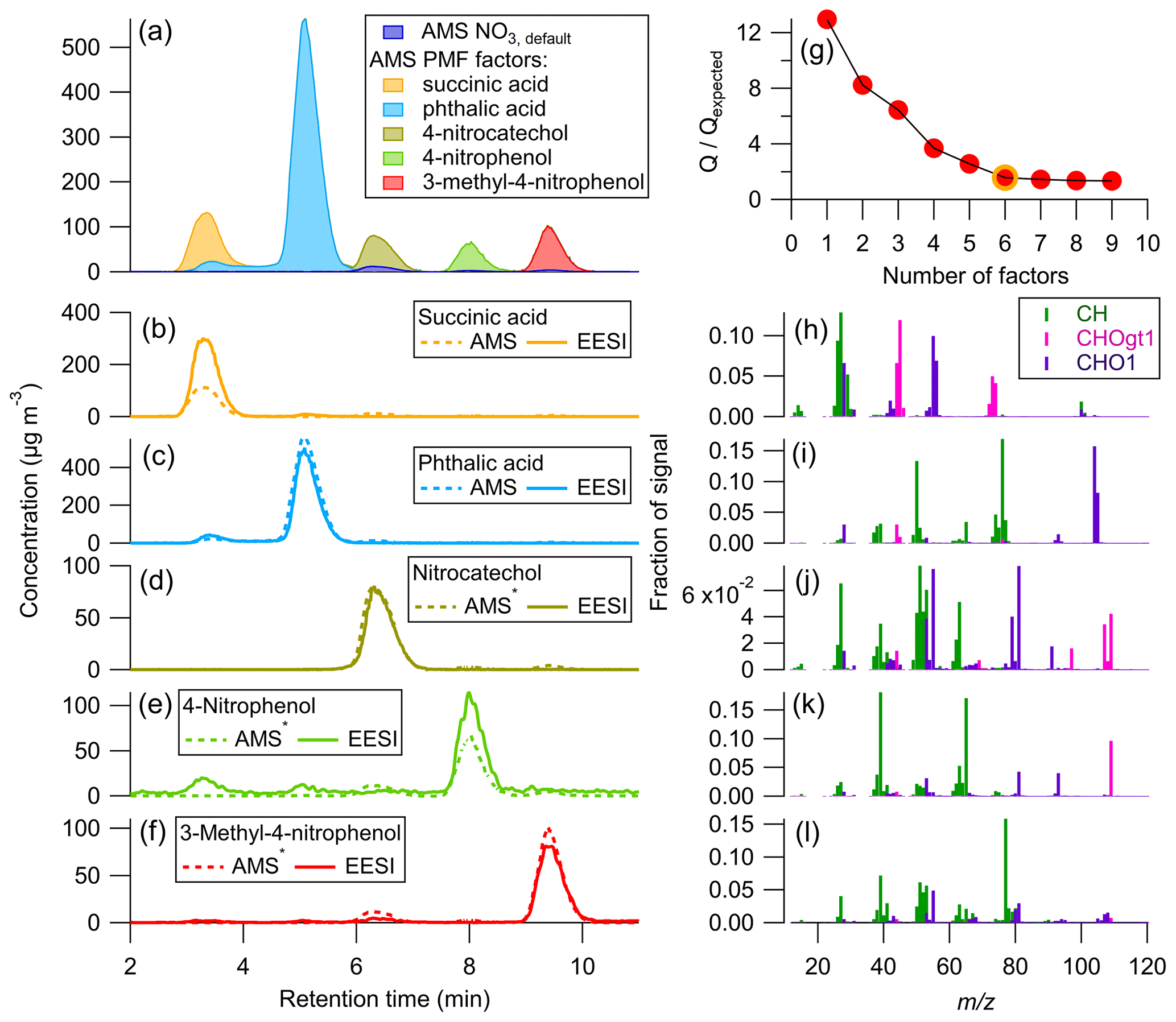
Figure 5 Time series for the AMS PMF solution: (a) stacked plot of each factor and AMS NO₃, (b–f) PMF factor with ${\mathrm{CF}}_x^{\mathrm{A}}$ applied to individual species, along with EESI concentrations. (g) $Q/Q_{\exp }$ vs. number of PMF factors, chosen solution circled in yellow. (h–l) Mass spectra (colored by associated AMS HR family) for each AMS PMF factor. A six-factor solution was chosen, with only five factors plotted here. The remaining factor was attributed to the background signal and was < 2 µg m⁻³ at all times. ^∗ AMS signal shown is OA + NO_3, default.

Figure 5a–f show excellent separation by PMF between the time series for each of the standards present in the mixture. This is likely due to the very different mass spectra for each species (Fig. 5h–l) as well as the time separation achieved by the HPLC. The mass spectrum for each standard was compared to the direct calibration mass spectra to confirm the AMS PMF factors were assigned correctly (Fig. S6 and Table S4). For all species, there was excellent correspondence, and the uncentered correlation coefficient (UC) between the mass spectral peaks was > 0.95.

Here, the ${\mathrm{CF}}_x^{\mathrm{A}}$ and ${\mathrm{CF}}_x^{\mathrm{E}}$ values are known for each pure standard (from direct calibrations). When applying the CF to individual species, the overall agreement between the AMS and EESI time series is comparable to that shown in Fig. 4. The AMS still underestimates succinic acid by a factor of ∼ 2 compared to the EESI, even after better separation is achieved with PMF. As discussed previously, this could be due to the mixing of the two species, which might change the viscosity or phase of the sampled aerosols compared to the pure species, which in turn could fundamentally change the ${\mathrm{CF}}_x^{\mathrm{A}}$ due to the change in CE. Whilst separation was achieved with PMF, PMF time series are likely more accurate for systems where different species have similar ${\mathrm{CF}}_x^{\mathrm{A}}$ (e.g., SOA mixtures from a single precursor and oxidant).

Figure 6 (a) Time series of AMS total OA (assumed ${\mathrm{CF}}_x^{\mathrm{A}}$ = 1.4), EESI HR ion, and absorbance (max = 4 × 10⁶, milli-absorbance units). (b–g) AMS PMF factor (assumed ${\mathrm{CF}}_x^{\mathrm{A},\mathrm{default}}$ = 1.4) and EESI HR ion for six calibrants. (h) Stacked PMF factor solution time series, (g) $Q/Q_{\exp }$ for AMS PMF solution, a nine-factor solution was chosen (yellow circle) with FPEAK = 0.2, and (j–o) AMS family colored mass spectra for six PMF factors. For levoglucosan and succinic acid, two factors were combined. The remaining factor was attributed to the background signal (< 2 µg m⁻³ at all times).

The AMS chromatogram for the mixture studied in Figs. 4 and 5 was mostly well separated without PMF. In order to assess the ability of PMF to separate AMS data for a more complex mixture, PMF was run on a different standard solution shown in Fig. 6.

Unlike the data shown in Figs. 3–5, the species run in the standard solution shown in Fig. 6 were not calibrated directly. Thus, Fig. 6 serves as a test of PMFs ability to resolve AMS data for complex mixtures, rather than a comparison of the calibration methods. Figure 6a shows the uncalibrated time series/chromatogram for the standards in the mixture. In contrast to the previous mixture, this solution contains five co-eluting peaks: levoglucosan, L-malic acid, citric acid, succinic acid, and a small fraction of the phthalic acid and its isomer. These five co-eluting peaks suggest that the application of only HPLC with the separation method being used here is not sufficient for these species, likely due to how polar they are. Further separation could be achieved by either changing the HPLC method (through the use of a normal phase chromatography, which uses for example a silica column) or running PMF on the AMS data.

Figure 6b–h show AMS PMF time series for the standards present in the mixture. In Fig. 6b, both the AMS and EESI levoglucosan peaks have different shapes. The EESI peak has a right tail, which is potentially due to the “sticky” (semi-volatile) nature of levoglucosan (Brown et al., 2021). The AMS peak has a sharp increase and slow descent and does not resemble a Gaussian (which is the approximate shape we expect eluting peaks to have). This is likely due to an imperfect PMF separation. Despite that, when comparing the mass spectra in Fig. 6j to the direct calibration mass spectra in Fig. S7, UC (Table S5) is 0.93, suggesting consistency between the two mass spectra.

L-malic acid and citric acid also co-elute with levoglucosan. For citric acid, L-malic acid, and levoglucosan, the mass spectra shown in Fig. 6j–l are somewhat similar. For L-malic acid and levoglucosan, $m/z$ 60 makes up some of the observed signal. While $m/z$ 60 is a known levoglucosan AMS ion, the direct calibration mass spectrum for L-malic acid also shows some signal at $m/z$ 60. The PMF mass spectrum for L-malic acid has a slightly higher ratio of $m/z$ 60 relative to the other ions, which could suggest that there is some mixing between the L-malic acid and levoglucosan factors. The assigned L-malic acid factor has a UC of 0.89 with the directly calibrated mass spectra, but citric acid was not directly calibrated for, and it is likely there is some overlap in the AMS factors between those three species. This was an especially complex solution for PMF to resolve due to the very similar retention times and mass spectra between these species.

As in Fig. 5, succinic acid, phthalic acid, and 4-nitrocatechol (Fig. 6e–g and m–o) are easily resolved when running PMF on the AMS chromatograms. This is likely due to both the retention time differences and the different AMS mass spectra for these three species. In Table 1, calibration factors are shown for levoglucosan, succinic acid, phthalic acid, and 4-nitrocatechol. ${\mathrm{CF}}_x^{\mathrm{A}}$ is known from the direct calibrations done in Fig. 4. During this experiment, only levoglucosan was cross-calibrated with a direct calibration; however, the multi-instrumental calibration value is highly affected by the shape of the AMS PMF factor associated with levoglucosan. Thus, the multi-instrumental calibration factor for levoglucosan is likely incorrect. The PMF factor stacked time series is shown in Fig. 6h. These results suggest that while PMF run on the AMS data does provide further peak resolution compared to HPLC alone, PMF cannot completely resolve all co-eluting peaks.

3.3 Combined application of the multi-instrumental calibration method and PMF on β-pinene + NO₃ SOA

In order to test the applicability of the proposed method to a complex real system, SOA from β-pinene + NO₃ was generated, collected on a filter, extracted, and analyzed with our multi-instrument system (per Sect. 2.1). This SOA system has been studied in depth previously, and 95 % of the SOA mass is composed of eight unique products, shown in Table 1 in Claflin and Ziemann (2018) and Table S6 here. Of the eight known products, we identified molecular ions that are attributed to a monomer ($m/z$ 268.1, assumed to be [C₁₀H₁₅NO₆–Na]⁺) and five dimers. Some of the dimers elute as different isomers, but the EESI HR ions observed corresponded to $m/z$ 451.2 ([C₂₀H₃₂N₂O₈–Na]⁺), $m/z$ 467.2 ([C₂₀H₃₂N₂O₉–Na]⁺), $m/z$ 483.2 ([C₂₀H₃₂N₂O₁₀–Na]⁺), and $m/z$ 499.2 ([C₂₁H₃₆N₂O₁₀–Na]⁺), all of which were identified in Claflin and Ziemann (2018). We also observed two additional ions, $m/z$ 388.2 and $m/z$ 465.2, whose structures remain unknown. To better compare the differences in the chromatogram obtained here vs. those shown in Claflin and Ziemann (2018), we compare the UV–Vis time series in Fig. S9. The chromatograms are similar, although their chromatogram had a slightly better resolution. Differences in observed species could potentially arise due to the age of the SOA extract used here (∼ 1 year) vs. the fresh SOA extract used in that study, fragmentation of species in the EESI (e.g., $m/z$ 388.2), or other experimental factors. For simplicity, the SOA peaks observed will be referenced by their associated EESI HR ion.

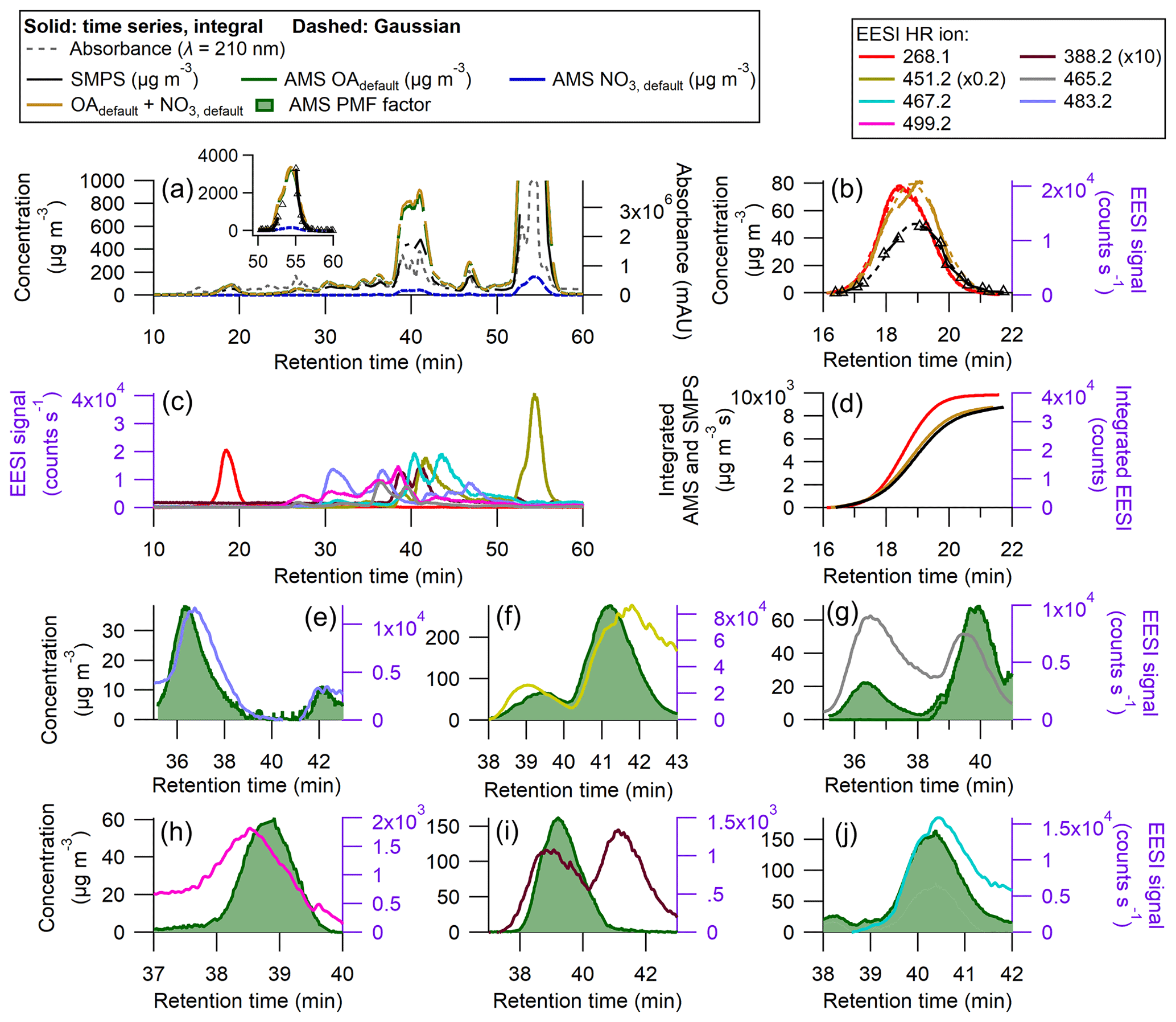
Figure 7 Results of an HPLC run for SOA from β-pinene + NO₃ (a) AMS, SMPS, and UV–Vis chromatograms (milli-absorbance units), with inset showing peak from 50–60 min. (b) Time series and Gaussian fits for the peak between 16 and 20 min (without using PMF), (c) EESI HR ions time series (d) time-integrated mass concentrations (ion signal) for AMS OA and NO₃, SMPS total mass, and EESI+ HR ion ($m/z$ 268.1). Panels (e)–(j) show some AMS PMF factors against measured EESI+ HR ions. Panels (g), (i), and (j) represent split AMS PMF factors for the measured EESI+ HR ions. The AMS PMF factors have a ${\mathrm{CF}}_x^{\mathrm{A}}$ ranging from 1.46–1.97 as shown in Fig. S3 and Table 2. Densities are applied to the SMPS data, shown in Fig. S8.

Figure 7a shows the full time series for the β-pinene system. Many of the peaks are not resolved enough to allow for the direct calculation of ${\mathrm{CF}}_x^{\mathrm{A}}$ and ${\mathrm{CF}}_x^{\mathrm{E}}$ using the SMPS as a the reference, as discussed in Sect. 2.7. The degree of peak co-elution is shown in Fig. 7c. There are two isolated peaks: $m/z$ 268.1 from 15–21 min and $m/z$ 451.2 from 52–58 min. The raw (and fitted) data are shown in Fig. 7b for the EESI ion measured at $m/z$ 268.1. The integrated fits are shown in Fig. 7d.

The EESI sensitivities for the overlapping peaks from ∼ 30 to ∼ 50 min were calculated by referencing the observed EESI signal to the AMS PMF time series. In Fig. 7e–j, AMS PMF time series that increased during the middle third of the run are shown alongside EESI HR ions. The full PMF solution can be found in Figs. S10–S12. AMS factors were matched with EESI HR ions based on the retention time and general shape of the time series. For some peaks, the retention times differ by up to 0.5 min. The complexity of this solution, as well as the similarities in the products' molecular structures, likely hindered the ability of PMF to fully resolve each individual product. For many of the overlapping peaks, the magnitudes of the individual AMS PMF factors are comparable.

${\mathrm{CF}}_x^{\mathrm{E}}$ and ${\mathrm{CF}}_x^{\mathrm{A}}$ are given for each identified species in Table 2. Many of the identified species have ${\mathrm{CF}}_x^{\mathrm{E}}$ in the same range as levoglucosan, within a factor of 3.

Table 2 EESI HR ion, ${\mathrm{CF}}_x^{\mathrm{E}}$ (counts s⁻¹ µg⁻¹ m³), ${\mathrm{CF}}_x^{\mathrm{E}}/{\mathrm{CF}}_{\mathrm{levo}}^{\mathrm{E}}$, and ${\mathrm{CF}}_x^{\mathrm{A}}$. ${\mathrm{CF}}_{\mathrm{levo}}^{\mathrm{E}}$ = 441.6 counts s⁻¹ µg⁻¹ m³. ${\mathrm{CF}}_x^{\mathrm{E}}$ was calculated using the AMS PMF [OA] × 1.05 (the average [NO₃] contribution was ∼ 5 %, Fig. S3).

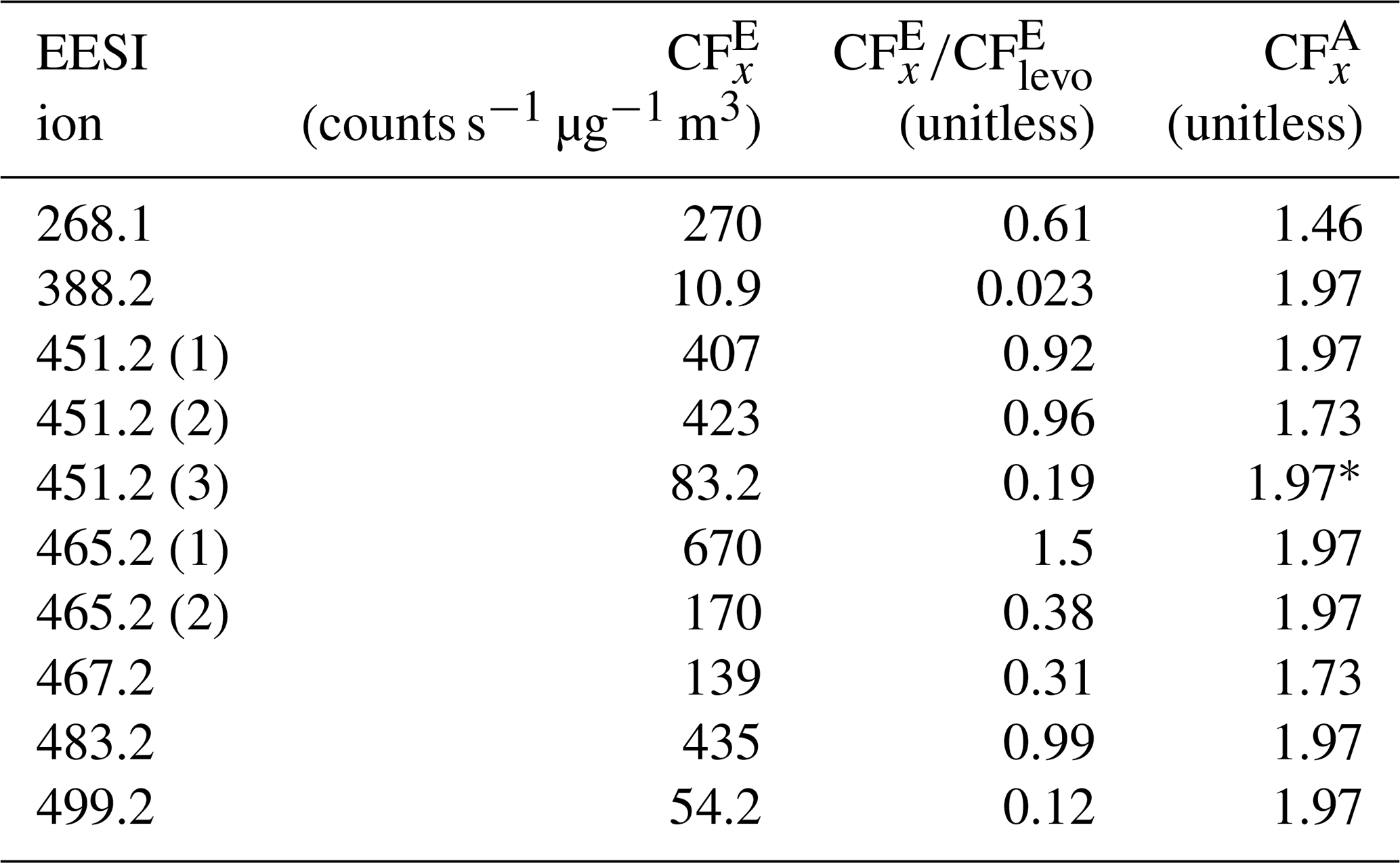
^∗ Incomplete SMPS data, assuming ${\mathrm{CF}}_x^{\mathrm{A}}$ = 1.97.

Some species, like the EESI HR ions measured at $m/z$ 388.2 and $m/z$ 499.2, have much lower EESI sensitivity than the other species. These species could be fragments of a larger parent ion, or they could be species that, for whatever reason, do not form a strong adduct with Na⁺. The ambiguity in the PMF factors may result in some errors in ${\mathrm{CF}}_x^{\mathrm{E}}$, but they are unlikely to fully explain the factor of 10 difference in sensitivity between the most and least sensitive β-pinene + NO₃ products. In future runs with slightly better chromatographic separation, a multivariate fit of individual factors vs. the SMPS may allow further constraining the quantification.

In this system, many of the products differ only by one or two oxygen atoms. In some cases, a carboxylic acid functional group replaces a ketone, whilst other molecules contain a cyclic ether, and some do not. The subtle differences in structure could influence the sensitivity with the EESI, as the oxygenated moieties may change the likelihood of forming a strong [M + Na]⁺ adduct. Further, some EESI HR ions eluted multiple times (e.g., $m/z$ 451.2). Claflin and Ziemann (2018) identified the structure of this ion for the third peak (shown in Table S6). However, this ion is measured twice more, from 38–43 min, which suggests the presence of isomers. Isomers can have different structures (shown in Table S6) and different ${\mathrm{CF}}_x^{\mathrm{E}}$. One example is $m/z$ 483.2, where one isomer has a ${\mathrm{CF}}_x^{\mathrm{E}}$ = 327.2 and a second isomer has a ${\mathrm{CF}}_x^{\mathrm{E}}$ = 54.2 counts s⁻¹ µg⁻¹ m³.

Despite differences in ${\mathrm{CF}}_x^{\mathrm{E}}$, ${\mathrm{CF}}_x^{\mathrm{A}}$ was more consistent. In Table 2, the AMS response to different SOA species formed from a single volatile organic compound (VOC) precursor varies only by 25 %. For the mixed peaks ${\mathrm{CF}}_x^{\mathrm{A}}$ was either 1.97 or 1.73, as discussed in Sect. S3 and shown in Fig. S3. For one of the isolated peaks, $m/z$ 451.2, the actual ${\mathrm{CF}}_x^{\mathrm{A}}$ was not calculated, due to a malfunction of the SMPS system between 54– 56 min. Individual peaks' Gaussian fits and integrated curves are shown in Fig. S13.

3.4 Discussion on the application of this method

In this paper, a novel technique was introduced that allows for the calibration of real-time mass spectrometers for individual species that cannot be obtained directly. This paper addresses the feasibility, performance, and limitations of this technique, all of which are necessary for any future use of this method.

The original purpose of this method was to calibrate species in SOA formed from laboratory chamber experiments. In many cases, the identity of the species was unknown, or the species could not be purchased as a pure standard. During those chamber experiments, SOA composition was measured in real-time with AMS, EESI, and SMPSs. SOA was also pulled through a Teflon filter, extracted in solvent, injected into the HPLC.

One application of this method would allow calculating yields for different SOA species produced from the oxidation of individual VOCs. This would allow for a better understanding of the chemical and partitioning mechanisms controlling the SOA composition and formation, along with providing information on which species are contributing the most to environmental and human health issues caused by SOA (e.g., higher light absorption or increased toxicity).

Another application is inferring calibration factors for important species in field data sets. This could be done by collecting filters to use with this method, including using ultra-performance liquid chromatography (UPLC) for higher resolution. Alternatively, if specific primary sources or SOA precursors are known to be important for a data set, those can be sampled in the lab to determine key species and their calibration factors.

One example of a field application is the FIREX-AQ field campaign, where the Jimenez Lab at the University of Colorado Boulder operated an EESI (Pagonis et al., 2021). During that campaign, direct calibrations were performed daily using either 4-nitrocatechol or levoglucosan. In the laboratory, these calibrations were also carried out daily, before chamber experiments and before running the HPLC calibration method. If species-specific sensitivities are obtained in the lab, then they can be ratioed to either 4-nitrocatechol or levoglucosan, providing the relative sensitivity of individual analytes. The relative sensitivity can be referenced to the sensitivities obtained in the field, allowing for the budgeting of ambient SOA for multiple species.

4 Conclusions

In this study, we introduced a novel multi-instrumental calibration method for EESI and AMS that uses HPLC and PMF to separate complex standard mixtures and SOA into individual species or subgroups of species present in the mixture. Our proof-of-concept test using individual pure standards demonstrated close agreement (within 20 %) between direct and multi-instrumental calibration factors, indicating this method's quantitative ability. In a second proof of concept using a mostly resolved standard mixture, EESI direct and multi-instrumental calibration factors agree within a factor of 2 for low-volatility species. We note that this method is not suitable for semivolatile species whose C^∗ is similar or higher than the concentration of aerosol sampled inside the SMPS DMA column. These results suggest that this method can be used to reliably determine species sensitivities for completely and mostly resolved chromatograms.

When HPLC alone failed to fully resolve individual analytes, PMF on AMS data successfully resolved individual analytes time series in a simple standard mixture. However, in more complex standard and SOA mixtures, while PMF provided some additional chromatographic separation, the PMF solution showed signs of factor mixing. This was especially evident in the β-pinene + NO₃ SOA mixture, which contained many similar analytes, resulting in a less well resolved PMF solution. While approximate EESI and AMS calibration factors were obtained, these sensitivities are affected by the inherent error in the PMF solution. In practice, while some mixtures may be adequately resolved by HPLC alone, AMS PMF can improve the chemical resolution of complex systems.

Future studies should prioritize improving the chromatography for the system of interest, potentially through changing the column type and/or mobile phase gradients, or using systems with higher intrinsic resolution such as UPLC (Kenseth et al., 2023). During the experiments shown in this article, we were limited to a C₁₈ column, which is primarily suited for separating less polar species. However, in the polar standard mixtures shown here and in scenarios involving significant oxidation and smaller precursor gases, the resulting products are likely too polar to be adequately separated by a C₁₈ column. In those experiments, a column with a polar stationary phase would allow for the separation of SOA components.

In conclusion, our method offers a valuable tool for quantifying EESI and AMS sensitivities in mixtures, especially pertinent for laboratory-generated SOA lacking pure standards or characterized by unknown isomeric forms. This technique can also be applied to other real-time aerosol mass spectrometers. To our knowledge, this technique stands as one of very few available methods for rapid calibration of EESI and AMS for SOA species that are unavailable as pure standards, emphasizing its significance in atmospheric research.