Impact of agricultural interventions on ammonia emissions and on PM_2.5 concentrations in the UK: a local and regional modelling study

The contribution of agricultural emissions of fine particulate matter (PM_2.5) poses significant health and environmental challenges, particularly in the UK where intensive farming activities contribute to elevated pollutant levels. This contribution includes direct emissions and PM_2.5 formed through chemical reactions from precursors such as ammonia (NH₃). The study aims to analyse the impact of a series of mitigation measures through emission scenarios (low, medium, high uptake) on the dairy, pig, and poultry sectors in 2030, mainly focusing on NH₃ emissions. Under the high-uptake scenario, NH₃ emissions could decrease by up to 13 % nationally, with reductions reaching as high as 20 % in certain regions. The Community Multiscale Air Quality (CMAQ) and the Atmospheric Dispersion Modelling System (ADMS) models were used. CMAQ allows one to understand the contribution made by agricultural NH₃ to secondary PM_2.5 at a regional scale, while ADMS is used to better understand near-field dispersion and the dilution of primary pollutants. Despite the impact of the changes in emissions due to the mitigation measures compared to the future baseline scenario, changes are not reflected on regional-scale PM_2.5 concentrations since the maximum modelled decrease was around 1 %–1.5 %. This finding is explained by an NH₃-rich atmosphere reducing the impact of these reductions in NH₃ emissions on mitigating PM_2.5 concentrations. Results from ADMS show that the NH₃ and PM_2.5 concentrations are quickly dispersed near the farms, highlighting the usefulness of local modelling in addressing impact studies on PM_2.5 formation near these sources. Indeed, for the five studied livestock farms, it has been found that 50 % of maximum NH₃ and PM_2.5 concentrations are located within a distance between 100 and 400 m, and up to 90 % of concentrations have decreased within 700 m. The study also demonstrates the complementary use of local and regional modelling in understanding PM_2.5 dispersion near agricultural areas. The comparison with ground-based measurements may suggest a non-representation of atmospheric processes in the PM_2.5 formation by CMAQ (with an underestimation of PM_2.5 concentrations by approximately 50 %). It underscores the need for integrated modelling approaches to guide mitigation strategies for both primary and secondary PM_2.5, as well as to improve our understanding of the chemical atmospheric processes involved in secondary inorganic aerosols.

1 Introduction

Air pollution from PM_2.5 (fine particulate matter with a mass median aerodynamic diameter < 2.5 µm) has been estimated to cause millions of premature deaths annually in recent years (Burnett et al., 2018; Kiesewetter et al., 2015; Lelieveld et al., 2015). PM_2.5 poses significant environmental and public health problems due to its ability to penetrate deep into the respiratory system, causing various health issues, including respiratory and cardiovascular diseases (Pope and Dockery, 2006). Therefore, mitigating this PM_2.5 pollution is a high priority for environmental protection in many regions, such as the European Union (EU) and in the United Kingdom (UK).

Among the various components contributing to PM_2.5 concentrations, ammonia (NH₃) has an important role in secondary particulate formation. In the atmosphere, NH₃ reacts with acidic compounds such as sulfuric acid (H₂SO₄) and nitric acid (HNO₃), forming ammonium sulfate ((NH₄)₂SO₄) and ammonium nitrate (NH₄NO₃), which are significant constituents of PM_2.5 (Seinfeld and Pandis, 2016; Wyer et al., 2022).

The UK presents a significant case for examining the influence of NH₃ on PM_2.5 levels due to its varied agricultural practices, transport-related emissions, and industrial activities. NH₃ emissions in the UK primarily originate from agricultural sources, particularly livestock waste and the application of fertilizers (Misselbrook et al., 2023). Indeed, the most recent figure from the UK National Atmospheric Emissions Inventory (NAEI) shows that agriculture accounted for nearly 87 % of total ammonia emissions in 2023 (NAEI, 2025). Direct soil emissions account for 52.7 % of total NH₃ emissions, followed by cattle at 25.9 %, waste at 9.5 %, other livestock at 4.8 %, poultry at 3.7 %, and combustion and production processes at 3.4 %. These emissions have been shown to vary seasonally and spatially, influencing the formation and distribution of airborne PM_2.5 concentrations (e.g. Wyer et al., 2022). Various mitigation measures (i.e. farm practices) have been developed to mitigate emissions of NH₃, such as covering slurry stores or using automatic scrapers in housing; however, reducing air pollution from agriculture remains challenging (Jenkins and Wiltshire, 2025).

Previous studies have highlighted the importance of understanding the interaction between NH₃ and PM_2.5 to inform regulatory measures and mitigate adverse health effects. For instance, the work by Vieno et al. (2014) demonstrated that reductions in NH₃ emissions could lead to significant decreases in PM_2.5 levels, especially in areas with large nitrogen oxide (NO_x) concentrations, suggesting that targeted strategies in NH₃ emission control could be effective in improving air quality. These results were confirmed by the study of Ge et al. (2023) – they showed that NH₃ reductions are more effective for regions or countries with better air quality, such as in the UK (compared to Asia, for example), in mitigating PM_2.5 concentrations. The impact of NH₃ emissions reduction is significantly more efficient with large emission reduction measures (Bessagnet et al., 2014), and abating NH₃ emissions can even be more cost-effective than NO_x for mitigating PM_2.5 air pollution (Gu et al., 2021). Conversely, other work such as Ge et al. (2022) and Pay et al. (2012) suggested that NH₃ emissions reduction may only lead to minor improvements in airborne PM_2.5 concentrations, especially in the UK since the UK is characterized by an NH₃-rich atmosphere. A study in the United States also showed that controlling NH₃ became significantly less effective for mitigating PM_2.5 in rural areas (Pan et al., 2024).

Due to the complexity of atmospheric chemistry, numerical air quality models such as chemistry transport models (CTMs) are commonly used to simulate these processes and assess the effectiveness of potential emission control strategies. CTMs such as the Community Multiscale Air Quality (CMAQ) model (Appel et al., 2021), developed and distributed by the US Environmental Protection Agency (EPA), is a cutting-edge numerical air quality model that comprehensively represents the emission, formation, destruction, transport, and deposition of numerous air pollutants, including PM_2.5 and its precursors. CTMs such as CMAQ are designed to calculate background concentrations, i.e. air pollutant concentrations at a km-scale spatial resolution (De Visscher, 2014).

Local dispersion models like the Atmospheric Dispersion Modelling System (ADMS) (Carruthers et al., 1994) can be utilized to provide detailed simulations of pollutant dispersion at a finer scale, such as 1 m. ADMS is particularly effective for assessing the impact of emissions from specific sources and understanding local air quality variations (Zhong et al., 2023). The combination of local dispersion models such as ADMS with CTMs allows a more comprehensive understanding of both regional and local air quality dynamics. Indeed, local modelling studies have shown their accuracy in determining the dispersion of pollution (Hood et al., 2018; Porwisiak et al., 2024; Zhong et al., 2023). ADMS is by default a steady-state (non-reactive) Gaussian plume model that predicts pollutant concentrations based on the assumption that both the vertical and horizontal dispersion of the continuous plume is represented by normal distribution around the plume centreline. However, due to the steady-state assumption, short-range estimates within 10 km are recommended (Environmental Protection Agency, 2020).

The aim of the study was to understand the impact of mitigation measures relating to livestock housing, and the storage and spreading of manures and slurries on PM_2.5 concentrations. This was part of an interdisciplinary project named AIM-Health, which included stakeholder engagements, measurement campaigns, air quality modelling, a health impact assessment, an economic study, and an ecosystem impact assessment. A companion study has already presented the impact of these policies on NH₃ concentrations and nitrogen deposition at a regional scale (Pommier et al., 2025). This study primarily focussed on measures to reduce emissions from housed dairy, pigs, and poultry, while emissions from other sources such as manufactured fertilizers were not within its scope. Three intervention scenarios were developed to model the impact on PM_2.5 concentrations nationally, based on differing uptake levels of the mitigation measures across the UK, with ranges covering from low, medium, and high. Additionally, local modelling was done to show how primary emissions of NH₃ and PM_2.5 disperse within the local vicinity (10 km) of farms included in this study.

Section 2 of this paper describes the methodology used for the scenario development and the air quality modelling (regional and local). The analysis on the modelled PM_2.5 concentrations is presented in Sect. 3. Section 4 discusses the results, and Sect. 5 gives the conclusions and perspectives.

2 Method

A series of mitigation measures related to livestock diet, livestock housing, and improved storage and spreading of manures and slurries were modelled to understand the impact on emissions from housed dairy, pigs, and poultry across the UK. The mitigation measures were modelled through scenarios that represented various levels of uptake (low–high) on these farms across the UK in 2030.

Whereas the regional modelling assumes a progressively higher national adoption of measures across these low to high scenarios, the local modelling applies only those mitigation strategies that are relevant to each individual farm. This approach is summarized in Fig. 1.

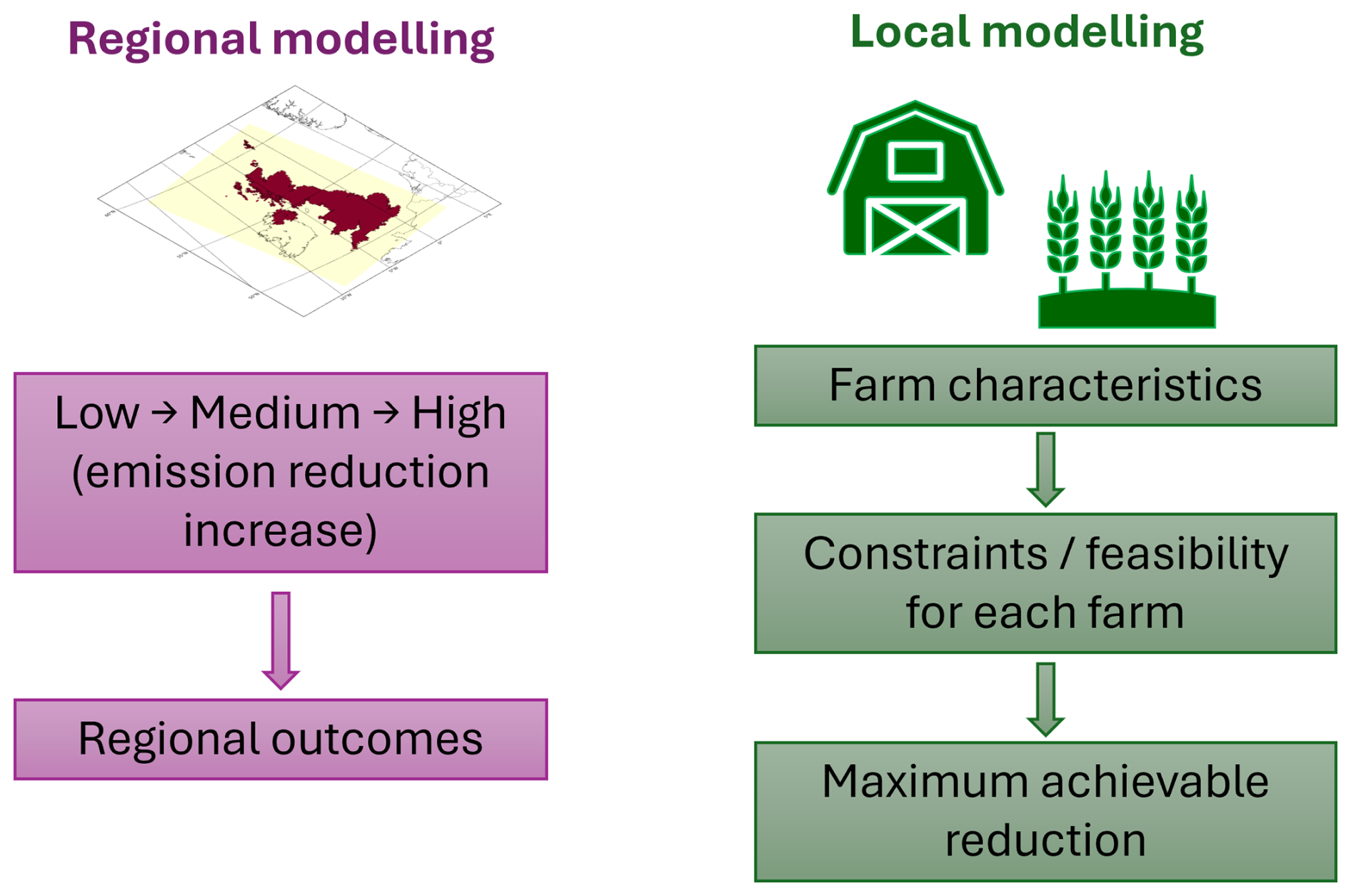
Figure 1 Schematic workflow for designing the emission scenarios.

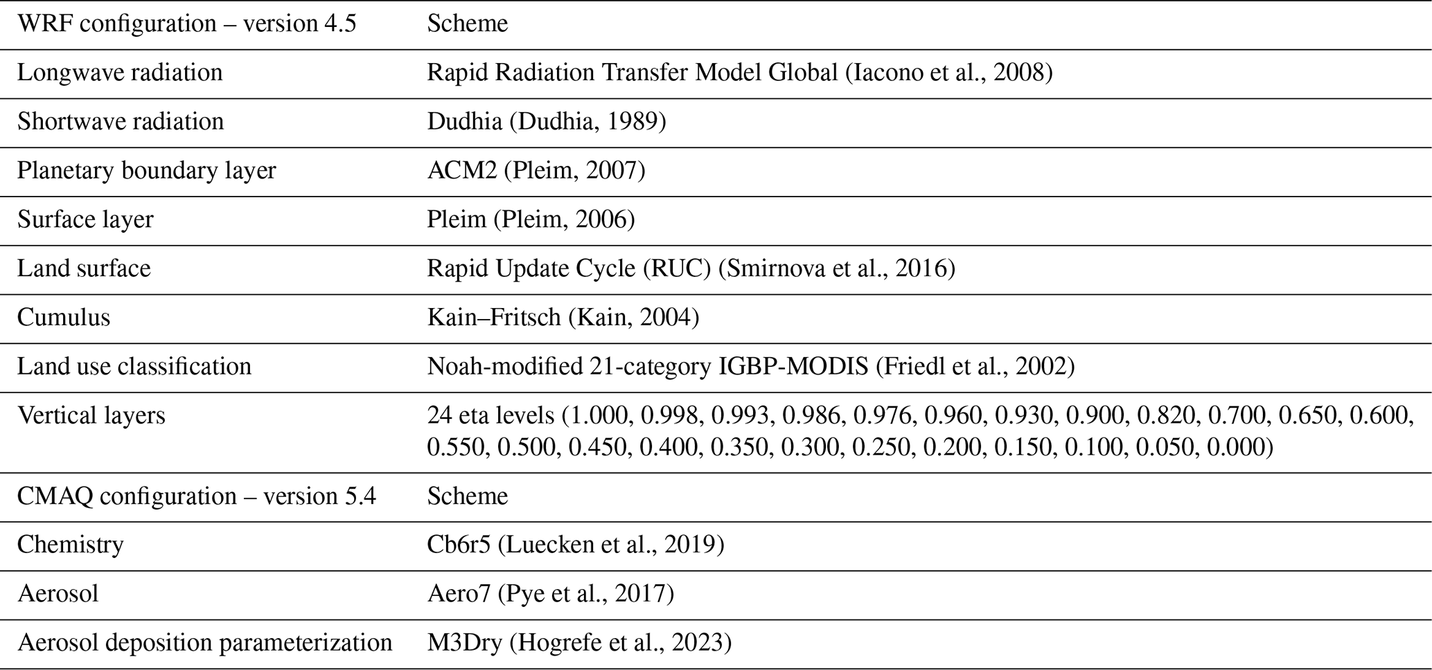
To undertake the study, the CMAQ model, has been used for the regional modelling and evaluated. CMAQ is a 3D Eulerian model, incorporating the effects of meteorology, emissions, land use, chemistry, and aerosol processes on modelled air pollution. It has been developed to represent the emission, transport, formation, destruction, and deposition of many air pollutants, including nitrogen dioxide (NO₂), ozone (O₃), and PM_2.5. The version used in this study is 5.4 (US EPA Office of Research and Development, 2022a; https://doi.org/10.5281/zenodo.7218076). This chemical-transport model requires input from a weather model, emissions, and the background atmospheric composition. For our work, the CMAQ model has been driven by meteorological fields from the Weather Research and Forecasting (WRF) model version 4.5 (NCAR, 2022).

For the local modelling, ADMS version 6 (CERC, 2024) has been used. ADMS is a steady-state Gaussian air dispersion model that incorporates air dispersion based on planetary boundary layer turbulence structure and scaling concepts, including the treatment of both surface and elevated sources, and both simple and complex terrain. This model allows the calculation of concentrations of atmospheric pollutants emitted both continuously from point, line, volume, and area sources, or intermittently.

2.1 Scenario development

The list of 20 mitigation measures were identified by the European Commission's Best Available Techniques (BAT) reference document for the intensive rearing of poultry or pigs (Santonja et al., 2017) and Defra's Code of Good Agricultural Practice (COGAP) for Reducing Ammonia Emissions (DEFRA, 2024b). The year 2030 was chosen due to being 10 years in the future from the start of the research study, therefore establishing a realistic timeline for the practical implementation of new activities on farms. These measures mainly focus on controlling NH₃ emissions and not on mitigating the primary PM_2.5 emissions from farming activities.

Three scenarios have been considered: low, medium, and high uptake, and compared to a baseline in 2030; this is defined in the rest of the document as low2030, medium2030, high2030, and base2030, respectively. The uptake scenarios were developed through stakeholder engagement with farmers and stakeholders (i.e. farm advisers, academics, and farmer representatives) to assess the realistic implementation of specific mitigation measures.

Each scenario includes all 20 mitigation measures; however, with varying percentages of uptake, a table presenting levels of uptake is presented in Appendix A, and a table with descriptions of the mitigation measures is given in Appendix B. The number of measures listed in Tables A1 and B1 differ because each measure appears only once in Table B1, whereas Table A1 includes measures multiple times when they apply to more than one livestock sector. The uptake rates were unique to each mitigation measure in each sector and were reflective of feedback received through engagement activities. The engagement activities included an online survey, focus groups, and one-on-one interviews with participants from the dairy, pig, and poultry sectors, along with those in other sectors that utilize manure or slurry. A total of 161 people took part in the activities. Full results and methodology are detailed in Jenkins and Wiltshire (2025).

Discussions in these activities were centred around understanding the current level of uptake and the benefits and barriers associated with the mitigation measures to determine a potential future uptake. If a mitigation measure was received positively, it was estimated to have a higher uptake compared to measures that were received negatively by participants. This was determined in the final level of uptake for each scenario. The future uptake did not take account of any potential changes to legislation that may have an impact, as this information is not known; additionally, there were no different uptakes for each part of the UK due to a lack of data.

To determine the emission reduction associated with each mitigation measure, the scenario modelling tool (SMT) was used (Ricardo EE, 2021). The SMT is a model for the management and analysis of complex scenarios of mitigation of air quality and greenhouse gas emissions from diverse sources in the UK, including agricultural sources. In this work, the model implements a mass flow model to track pollutant transfer between each of the locations on a farm, to correctly reflect the cascade of mitigation effects along the manure management chain.

The SMT calculates the effect on emissions of each scenario by adding measures with emission reduction values and uptake rates. It allows one to design mitigation measures using the effect on emissions (as a percentage of reduction), cost, and targeting (the point in the agricultural system/manure management chain at which the effect on emissions is felt). Uptake rates are used in the SMT, allowing for the uptake of each measure to be reflected as a percentage of a cohort of farms (e.g. fixed slurry cover can be applied to 15 % of dairy farms). It is worth noting that the cost impact of the measures is not discussed in this study.

There are different ways that the various types of measures are calculated in the SMT. In this study, “Emission” and “Reduction” measures were used. “Emission” measures directly reduce the pollutant emission factor at a location on a farm. This type of measure represents changes in practice or technical solutions, and is not typically used where a measure represents a change in the overall management system. “Reduction” measures reduce the quantity of a source of emissions (e.g. the number of animals in housing or the quantity of excreta in housing). This reduction is reflected in emissions occurring at all associated locations. In this study, the only “Reduction” measures used related to extended grazing on dairy farms and low protein diets in dairy, pig, and poultry farms. For the low protein diet measures, the quantity of excreta was reduced, while for the extended grazing, the quantity of managed solid and liquid manure was reduced. All other measures were implemented as “Emission” measures, directly reducing the emission factors at relevant locations.

The SMT comes with a default library of mitigation measures and associated emission reduction factors. These emission reduction factors have been calculated based on empirical evidence and published scientific literature (primarily UK based), and with reference to relevant international studies and the UNECE Task Force for Reactive Nitrogen Ammonia Abatement Guidance Document (Bittman et al., 2014). The mitigation impact of these measures from the SMT is verified for accuracy by comparison with data from the Agricultural Ammonia and Greenhouse Gas Inventory (AAGHGI) (Misselbrook et al., 2023).

Eleven measures that were included in the modelling in this project were not included in the predefined measure library. To determine how to reflect these 11 measures in the SMT (including what stage(s) in the agricultural system the measure is relevant to and if it is an “Emission” or a “Reduction” measure), as well as to confirm the emission reduction potential of these measures, COGAP, BAT, and expert knowledge were used. This information was added to the SMT using the “Measure” function as outlined above.

The calculation of measure effect takes account of measure interactions, including the order of implementation and exclusivity, and this employs the principal of maximum overlap of uptake and a multiplicative effects model, in line with similar earlier models such as the National Ammonia Reduction and Strategies Evaluation System (NARSES) (Webb et al., 2006; Webb and Misselbrook, 2004). Baseline emission data come from the AAGHGI (Misselbrook, et al., 2023). The data set for the year 2019 was used as baseline as it was the most recent submission at the time of running the scenarios.

2.2 Regional modelling: CMAQ

2.2.1 Model set-up

The CMAQ model, calculating the pollutants' concentrations and depositions at an hourly resolution, was set up using the same vertical and horizontal grid structure as for WRF, modelling the meteorology. Atmospheric chemistry was simulated using the carbon bond mechanism (CB06r5) (Luecken et al., 2019) combined with the aerosol mechanism using the 7th generation aerosol module (AERO7) (Pye et al., 2017). The dry deposition of gaseous species is simulated utilizing deposition velocity and the M3Dry aerosol deposition parameterization (Hogrefe et al., 2023). The configurations of the WRF and CMAQ models are given in Table 1.

Table 1 Summary of the WRF and CMAQ modelling settings.

A nested modelling approach has been employed, dividing the broader geographic area into smaller domains to enhance the spatial resolution. This hierarchical structure enables a more accurate representation of variations in emissions and meteorological conditions. The outer domain, covering Europe, uses a horizontal resolution of 50 km (EU50), while the inner domain focuses on the UK with a finer resolution of 10 km (UK10), as illustrated in Fig. 2.

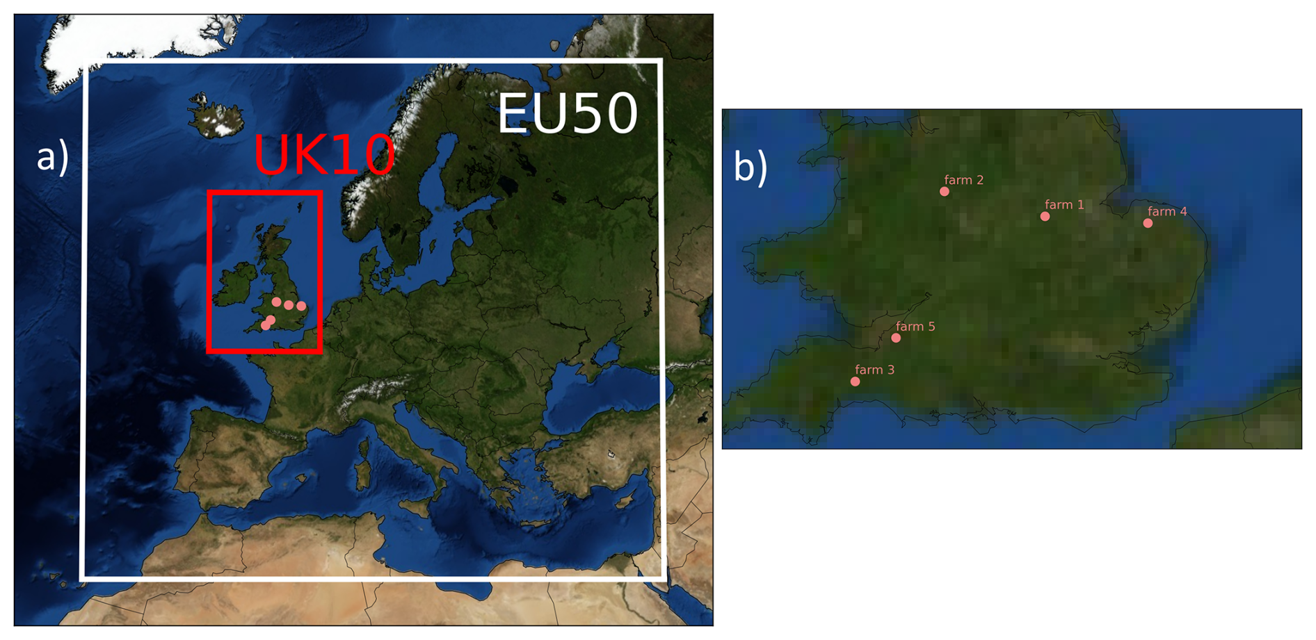
Figure 2 (a) Regional nested modelling domains and location of the studied farms, shown with the matplotlib NASA Blue Marble image used as an illustration. The white box corresponds to the European domain at 50 km × 50 km horizontal resolution (EU50) and the red box to the UK domain at 10 km × 10 km horizontal resolution (UK10). Each farm is shown with a pink coral circle. (b) Zoom on the location of each studied farm with their corresponding ID. The details of the farms are provided in Table 2.

The air quality simulations were carried out using meteorological data from 2019. This year was selected as the reference because it is classified as a typical meteorological year in the UK (see Pommier et al., 2025, and references within), and 2019 was also the most recent UK emissions year at the beginning of the project. This historical 2019 simulation has been used for model performance evaluation prior to the analysis of the future predictions with the scenarios. The future scenarios focussed solely on change in emissions, and no climate projection has been undertaken. Consequently, there is no analysis on changes in meteorological conditions.

The use of a single-year meteorology is a common approach in emission-driven scenario assessments. Nevertheless, interannual meteorological variability can influence secondary PM_2.5 formation and dispersion, meaning that results based on 1 year may not capture the full range of possible outcomes. As the study is designed to evaluate relative differences between emission scenarios under consistent meteorological conditions, the scenario-to-baseline contrasts are expected to be less sensitive to this limitation.

The regional simulation started with a spin-up period of 2 weeks. The simulation set-up follows a “forecast-cycling” approach, where the output fields from each run were used to initialize the simulation for the following day. This process has been applied continuously throughout the entire year of 2019 for both the EU50 and UK10 domains. The initial and boundary conditions for the outermost domain (EU50) were created using hemispheric CMAQ outputs for the year 2016 provided by the US EPA (US EPA Office of Research and Development, 2022b). Subsequently, the CMAQ concentrations computed in the EU50 domain were used as boundary conditions for the nested UK10 domain.

2.2.2 Emissions

The anthropogenic emissions data from the European Monitoring and Evaluation Programme (EMEP) (CEIP, 2022) were post-processed into 50 × 50 km resolution to populate our EU50 domain in CMAQ. The UK anthropogenic emissions, including from agriculture, were based on the gridded emissions from the UK National Atmospheric Emission Inventory (NAEI) for 2019 (Churchill et al., 2021). The NAEI provides gridded emissions data at a 1 km × 1 km resolution, which was post-processed to match the 10 km × 10 km resolution of the UK10 domain. Additionally, the 2019 large point source emission inventory was used to vertically distribute emissions in the CMAQ grid.

The baseline 2030 future scenario for the EU50 domain was based on the EMEP gridded emissions for 2019 and scaled with the factors provided by the GAINS ECLIPSE (Greenhouse Gas and Air Pollution INteractions and Synergies – Evaluating the Climate and Air Quality Impacts of Short-Lived Pollutants) V6b Baseline CLE scenario (IIASA, 2019).

With the exception of the UK base2030 scenario, all UK scenarios incorporate the same set of measures. The increasing adoption of these measures across the low2030, medium2030, and high2030 scenarios reflects progressively higher ambition in reducing air pollutant emissions, as described in Sect. 2.1.

Figure 3 shows the total UK anthropogenic emissions as used in CMAQ and highlights the main changes in these emissions for the different scenarios. Since the mitigation measures mainly tackle the NH₃ emissions, this explains the large decrease calculated for this pollutant. As explained in Pommier et al. (2025), the reduction in NH₃ emissions could reach up to 20 %, 22 %, and 24 % in certain regions under the low2030, medium2030, and high2030 mitigation scenarios, respectively. It is noteworthy that the UK NH₃ emissions are mainly dominated by the February–April period, as shown in Fig. S1 in the Supplement, and in Hellsten et al. (2007). Marais et al. (2021) reported an additional July peak associated with dairy cattle farming, based on satellite observations, alongside the spring peak. In contrast, the Emissions Database for Global Atmospheric Research (EDGAR) applies a uniform temporal profile for agricultural NH₃ emissions in the UK in its latest inventory version (EDGARv8.1: https://edgar.jrc.ec.europa.eu/dataset_ap81#p1m, last access: 2 November 2025).

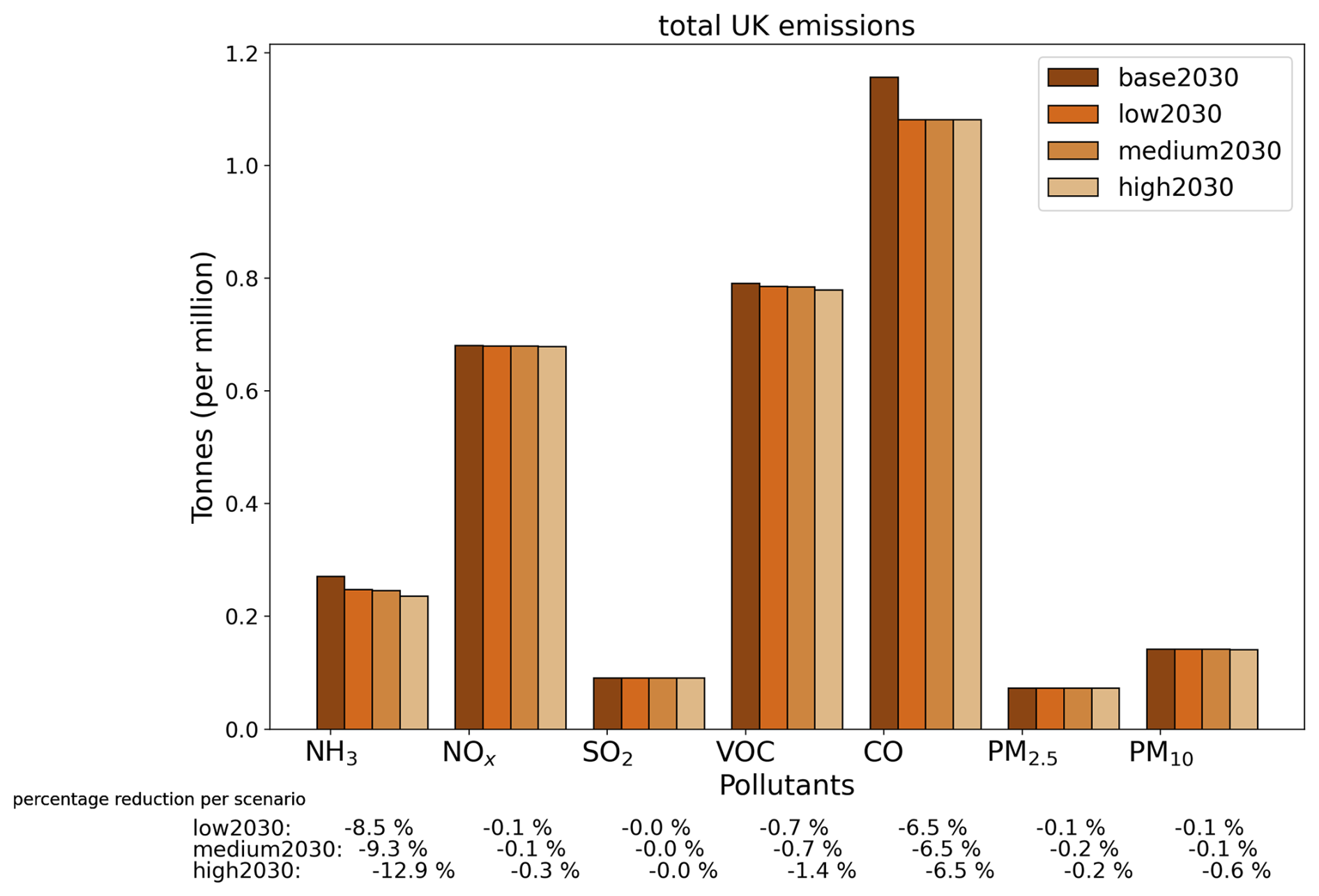
Figure 3 Total UK anthropogenic emissions in tonnes for the different scenarios used by CMAQ for NH₃, NO_x, SO₂, VOC, CO, PM_2.5, and PM₁₀. The relative difference for the low2030, medium2030, and high2030 scenarios compared to the base2030 are given below each corresponding bar.

A constant decrease in carbon monoxide (CO) is predicted across all scenarios. Unlike other pollutants, this trend is influenced not only by the selected mitigation measures but also by the scope of the SMT model, which does not fully capture all future CO emission sources. Slightly larger reductions in emissions are calculated for the high2030 scenario for volatile organic compounds (VOCs) and the coarse PM (PM₁₀, PM with an aerodynamic diameter lower than 10 µm), while the changes in NO_x and PM_2.5 remain limited and null for sulfur dioxide (SO₂).

CMAQ also calculates biogenic emissions with an online module incorporated in the model. This uses the Model of Emissions of Gases and Aerosols from Nature (MEGAN) version 3.2 (Guenther et al., 2020). CMAQ also calculates windblown dust (Foroutan et al., 2017) and sea spray emissions (Gantt et al., 2015; Kelly et al., 2010) with online modules. These emissions are identical in all scenarios.

2.3 Local dispersion modelling: ADMS

2.3.1 Model set-up

For the local modelling, meteorological data sets were procured from National Oceanic and Atmospheric Administration (NOAA) weather stations ranging from 6 to 25 km for farms in this study. Where data capture was insufficient, gap filling was performed to ensure coverage exceeded 85 % for all parameters, including wind speed, wind direction, cloud cover, temperature, and precipitation. Data filling involved selecting the most representative NOAA station for each farm, and where gaps were present in its data set, missing values were supplemented using data from the next most representative station. This approach ensured a more complete and more reliable data set for modelling. The year 2019 was selected as this year is consistent with the existing baseline year of the regional model.

Each farm, situated in a different region of the UK (Fig. 2), away from major roads and industrial areas, had a 15 km × 15 km points grid centred at the farm with a 100 m resolution. This was overlayed with the CORINE Land Cover 2018 100 m data (European Environment Agency, 2019) to extract map codes for each grid point. The land use classifications were associated with a surface roughness ranging between 0.04025 (water) and 1.3 (urban areas) in Aermet, the meteorological pre-processor for Aermod (Support Center for Regulatory Atmospheric Modeling, 2017, Appendix W Final Rule). NH₃ deposition was considered by using deposition velocities that vary depending on the surface. The deposition velocity values used for NH₃ vary between 0.02 m s⁻¹ for lower plants (lowland shrubs, grassland) and 0.03 m s⁻¹ for higher plants (woodlands) (Natural Resources Wales, 2021). Plume depletion was turned on in ADMS; this means that atmospheric concentrations of NH₃ and PM_2.5 decrease due to dry and wet deposition.

The requirement for complex terrain was established using the Environment Agency's 1m lidar data (DEFRA, 2023) to see if it met Defra's Local Air Quality Management modelling requirement (> 1:10) (DEFRA, 2022) for any of the farms. None of the farms displayed a terrain of 1 : 10 or above, and so complex terrain was omitted from the model.

ADMS can include buildings to simulate the impact of building downwash for point sources only, air recirculation leeward (downwind) of the building. Buildings within a distance three times the mechanical ventilation stack height were included to estimate the potential of increased concentrations very close to the source. This distance is a more conservative threshold than the Good Engineering Practice (GEP) criteria to allow for differences in building shape, wind direction, and wake effects, improving the accuracy of near-field dispersion modelling. The US Clean Air Act (US Environmental Protection Agency, 1985) sets a threshold at 2.5 times the height of the nearest structure, measured from ground level at the base of the stack.

The CMAQ modelled concentrations for the corresponding grid cells of the UK10 domain were used as background concentrations for NH₃ and PM_2.5. Indeed, the concentrations calculated by CMAQ or other CTMs with a somewhat coarse resolution are mostly representative of the background conditions.

2.3.2 Emissions

The emissions in the regional modelling have been calculated with the SMT, based on national emissions, whereas the local modelling has used a combination of emission rates derived from measurements undertaken as part of this project (Leonard and Wiltshire, 2025). In the absence of measured emissions, the Simple Calculation of Atmospheric Impact Limits (SCAIL) agricultural emission inventory (Hill et al., 2014) has been used.

The local modelling has focussed on five farms, chosen to represent the locations covered by the measurement campaign. These farms have remained anonymous for the study. Details on the farms included in local modelling – such as livestock type, number of sources, those that include measured or SCAIL emission inventories, and mitigation – have been detailed in Table 2.

Table 2 Farms included in local dispersion modelling. The text in italics, like “manure piles”, is the mitigation category.

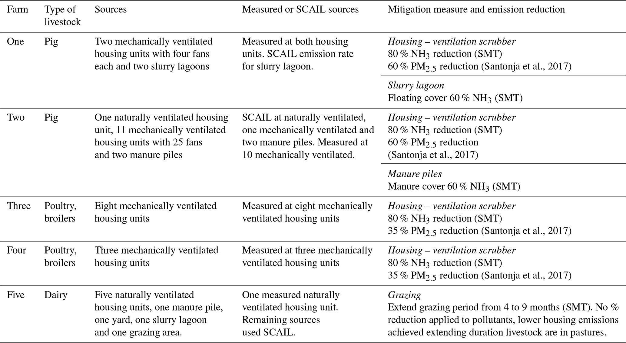
These farms have very high reductions in emissions because of their nature and the impact of specific measures (Table 2). However, overall, at a national level, the reductions are on average more modest, even if these farms are located where larger reduction in national NH₃ emissions were calculated (Pommier et al., 2025). In the local modelling, the emission reduction scenario reflects the maximum achievable reduction at the individual farm level depending on their characteristics, whereas the regional modelling evaluated a range of progressively increasing reduction scenarios (Fig. 1).

It is noteworthy that the measurement campaign was conducted during a challenging period, beginning with the onset of the COVID-19 pandemic at the beginning of the project, which significantly affected the recruitment of farms for fieldwork. Engagement with pig farms was particularly difficult due to severe abattoir delays – partly linked to the UK's departure from the European Union – which led to overcrowding on farms. These factors caused substantial delays in recruitment, further compounded by the withdrawal of two participant farms that had to be replaced, and operational issues at another farm that prevented the collection of usable data. Additionally, concerns about infection risks – both from COVID-19 and general biosecurity – limited access to measurement equipment. This led the study to focus on these five farms. While some farms had data collected for only part of an animal cycle (requiring assumptions about how representative the results were), the study still gathered high-quality comprehensive data from these five distinct locations.

The local dispersion modelling for all studied farms uses the same methodology, except for the development of the emission rates, which was unique to each farm depending on the availability of activity and monitoring data from farms. However, farm activity and monitoring data were consistently reviewed across each farm, with the final data used varying to reflect the level of detail available.

Detailed questionnaires, interview results, and pollutant (NH₃ and PM_2.5) measurements collected from each farm in this study were reviewed to establish the ADMS source type representation such as point, volume and area, and extent of time-varying profile to apply. The primary emission data used in the modelling have used the same quality assurance protocol detailed in the measurement study (Leonard and Wiltshire, 2025), with monitoring data being processed into hourly averages to reflect the hourly meteorological limitations of ADMS. The measurement, questionnaire, and interview results were used to establish existing emission profiles, and any existing mitigation measures to lower NH₃ or PM_2.5 were reflected in the baseline. However, none of the mitigation measures recommended in this study (Jenkins and Wiltshire, 2025) were in place at farms (Leonard and Wiltshire, 2025). An order of preference for time-varying emission profile development has been implemented. The most preferred to least preferred was defined as below.

Preferred emission profile – unique calculation for every hour in year

An emission rate (g s⁻¹) for every hour in a year is the most detailed emission input option in ADMS 6 (CERC, 2023), as emission measurements at farms were undertaken for periods during 2022 and 2023 did not represent a full year of measured emissions from sources. As a result, the most detailed option available for each farm would be to develop an emission rate (g s⁻¹) for every hour in the animal cycle, then extrapolate this over a year based on reports of all the animal cycles in a year. There was only sufficient monitoring and animal cycle data for each hour to have an emission rate at farm four (poultry). As there are only housing emission sources at farm four, every source on this farm was based on an individually calculated emission rate for every hour in a year.

Second emission profile preference – annual-average emission rate for each hour in a day

The next level of detail available to develop time-varying emission profiles at each farm was to calculate annual-average hourly emission rates (g s⁻¹) for the application of a diurnal profile in local modelling. This was applied to sources on farms one (pig), two (pig), three (poultry), and five (dairy) with measurement data. At pig farms one and two, this profile was applied to housing units with measurement data but also to housing units based on the SCAIL emission inventory as the profile was considered relevant. At farm three (poultry), a diurnal profile based on annual average hourly emission rates (g s⁻¹) was applied to all housing units. At farm five, the milking and loafing area was the only building where emission measurements were taken and the only one for which a diurnal profile was applied. These loafing areas were non-passageway, non-feeding spaces where cows can lie down and move freely, allowing them to express natural behaviours such as grooming and heat detection. Grazing areas and cattle housing were assigned two distinct emission rates to reflect seasonal differences between periods when cattle are grazing and when they are housed.

Third emission profile preference – constant emission rate for all hours in a year

The lowest level of detail occurs where no measurement or activity data were available to understand how annual emissions should vary throughout the day and/or year. In this situation, annual emissions were divided by the number of seconds in a year, resulting in a constant (g s⁻¹) for all hours in a year. No diurnal profile was applied to slurry and manure lagoons at farms one and two. At farm five (dairy), no diurnal profile was applied to the yard, slurry lagoon, or manure piles.

Information on emission sources, including dimensions, fan height, diameter, and exit velocity, were derived from farmer data requests and interviews. Housing temperature data were derived from either farm-owned temperature sensors if available or from project monitoring equipment. Hourly emission rates of NH₃ and PM_2.5 were calculated for each hour of the animal (flock) cycle or for the full measurement period, using Eqs. (1) (NH₃) and (2) (PM_2.5) (Phillips et al., 1998). All calculations were performed on an hourly average basis. The NH₃ emission rate was calculated as

$$\begin{array}{}\text{(1)}& {\text{ER}}_{{\mathrm{NH}}_{\mathrm{3}}}=C_{{\mathrm{NH}}_{\mathrm{3}}}\times Q\times R_{\mathrm{molecular}}\times c_{\mathrm{mass}},\end{array}$$

where ER${}_{{\mathrm{NH}}_{\mathrm{3}}}$ corresponds to the NH₃ emission rate (g s⁻¹), $C_{{\mathrm{NH}}_{\mathrm{3}}}$ is the hourly average NH₃ concentration (ppb), Q is the ventilation volumetric flow rate (m³ s⁻¹), R_molecular is the conversion factor from parts per billion to mass concentration based on the molecular weight and molar volume of NH₃, and c_mass is the conversion constant (10⁶).

The PM_2.5 emission rate was calculated as

$$\begin{array}{}\text{(2)}& {\text{ER}}_{{\mathrm{PM}}_{\mathrm{2.5}}}=C_{{\mathrm{PM}}_{\mathrm{2.5}}}\times Q\times c_{\mathrm{mass}},\end{array}$$

with ER${}_{{\mathrm{PM}}_{\mathrm{2.5}}}$ being the PM_2.5 emission rate (g s⁻¹), $C_{{\mathrm{PM}}_{\mathrm{2.5}}}$ the hourly average PM_2.5 concentration (µg m⁻³), Q the ventilation volumetric flow rate (m³ s⁻¹), and c_mass the unit conversion factor from micrograms to grams (10⁶).

For instances where emission rate values could not be calculated, the SCAIL emission inventory was used. SCAIL emission rates are provided as kg m⁻² or kg per animal place per year; as a result, the area of sources and number of livestock were used in this equation to derive NH₃ and PM₁₀ kg yr⁻¹. SCAIL emission rates are in PM₁₀. This was converted into PM_2.5 by looking at the ratio between PM_2.5 and PM₁₀ at Defra's Automatic Urban and Rural Network (AURN) rural background monitoring stations available at the UK AIR platform (DEFRA, 2024a) to derive a factor of 0.58. As the farms are located at different locations across the UK, an average value derived from multiple AURN stations was used for simplification, and, because the analysis considers annual concentrations, a fixed non-time-dependent conversion factor was applied. This assumed ratio (0.58), derived from background AURN observations, lies within the range typically reported for agricultural sources (Gladding et al., 2020), even if lower values were found by Demmers et al. (2010) (0.16 for broilers, 0.26 for free-range layers, and 0.41 for caged layers). A high variability in PM_2.5/PM₁₀ emission factors for UK poultry farms was also highlighted in a review study (DEFRA, 2012).

The measured emission rates were adjusted using Eq. (3) for comparison with SCAIL annual emissions (kg yr⁻¹). A livestock-type dependent emission rate was applied to each fan of the corresponding farm buildings to obtain the total emission from the farm buildings and therefore can be scaled up using the building volume:

$$\begin{array}{}\text{(3)}& \text{EF}=\text{ER}\times V_{\mathrm{building}}\times c_{\mathrm{mass}}\times c_{\mathrm{time}},\end{array}$$

with EF being the emission factor (kg yr⁻¹), ER the hourly average emission rate (µg (m³ h)⁻¹), c_mass the conversion constant (10⁹), and c_time the time conversion constant (24 × 365).

Mitigation scenario emission calculations

In the mitigation scenario, each emission source and associated percentage reduction from mitigation, detailed in Table 2, were applied to emission rates (g s⁻¹). For example, acid scrubbers are an applicable treatment of ventilated air at the farm one animal housing, and the emission rate (g s⁻¹) is multiplied by 0.2 and 0.4 to reflect the proposed 80 % and 60 % reduction in NH₃ and PM_2.5, respectively.

In summary, emission inputs from different data sources were harmonized before their use in ADMS by converting all source terms to a consistent pollutant-specific emission format. Farm-specific measurements were used preferentially and combined with hourly ventilation rates to derive hourly NH₃ and PM_2.5 emission rates. Where measurements were unavailable, SCAIL emission factors were converted to source-specific annual emissions using source area or livestock numbers, and SCAIL PM₁₀ emissions were converted to PM_2.5 using a fixed factor.

Temporal allocation was harmonized separately from emission magnitude: where appropriate, SCAIL-derived housing emissions were assigned a measured diurnal profile from a comparable farm source, while sources lacking supporting activity or measurement data were assigned constant annual-average emissions. This hierarchy also reflects relative confidence in the inputs, with fully measured hourly emissions considered most robust and fully inventory-based annual-average emissions the most uncertain.

3 Change in PM_2.5 concentrations

3.1 Regional scale

3.1.1 Evaluation of the historical simulation

The modelled concentrations have been evaluated using the historical simulation in 2019. Only PM_2.5 measurement data for rural background sites with at least 75 % data capture in the year are used to avoid bias. The observations were downloaded from the UK AIR platform. This represents a total of 48 stations. The CMAQ annual map and the comparison with the observations at the measurement sites are shown in Fig. 4. The statistics used in this evaluation are described in Appendix C.

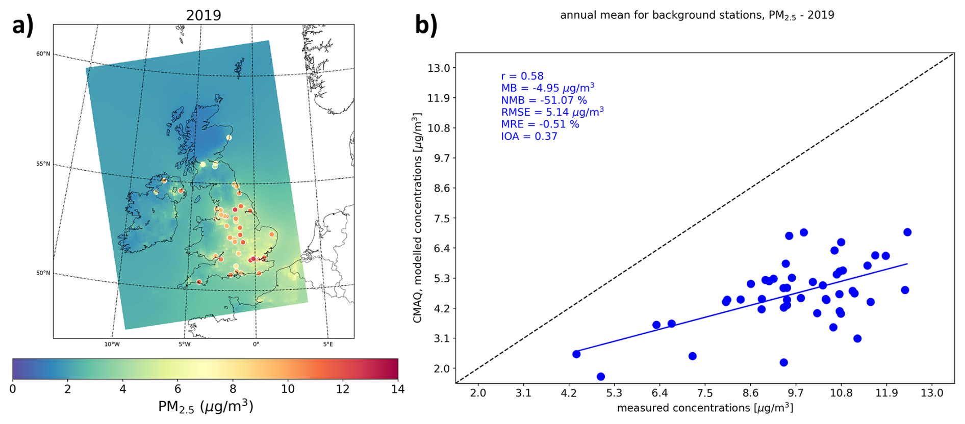
Figure 4 (a) Spatial distribution of annual mean PM_2.5 concentrations in µg m⁻³ calculated by CMAQ at 10 km resolution in 2019. The measured concentrations at the monitoring stations are shown with the coloured circles. (b) Comparison between these annual measured concentrations with the modelled values in 2019. Only the background stations with a data capture higher than 75 % are used. Insert values are the Pearson correlation coefficient (R), the mean bias (MB), the normalized mean bias (NMB), the mean relative error (MRE), the root mean square error (RMSE), and the index of agreement (IOA). The blue line represents the linear fit and dashed black line the 1 : 1 slope.

While the comparison shows a fair agreement in the correlation (r ∼ 0.6), a clear underestimation in the modelled concentrations is calculated (mean bias (MB) ∼ −5 µg m⁻³; normalized mean bias (NMB) ∼ −51 %, mean relative error (MRE) ∼ −0.5). This approximate 50 % underestimation in the modelled PM_2.5 concentrations mirrors the uniform 50 % increase in NH₃ emissions (and 60 % decrease in SO₂ emissions) applied by Kelly et al. (2023) and Marais et al. (2023), using a similar emissions inventory (NAEI for the year 2019) in their simulations to obtain a reasonable agreement in their calculated PM_2.5 concentrations with their global CTM (r = 0.66, NMB = −11 %). However, it is worth noting: a sensitivity simulation by increasing our UK NH₃ emissions by 50 % was also tested. Despite this large change in the 2019 NH₃ emission, no real improvement in the comparison with the observations was found (Fig. S2). This confirms the finding in Pommier et al. (2025) showing that NH₃ is not “limiting”, thus NH₃ emission changes will have a negligible impact on mitigating secondary inorganic aerosols (SIA) formation at the regional scale. Kelly et al. (2023) also explained that with NH₃ being in excess, the emissions scaling applied to NH₃ to resolve differences between top-down and bottom-up emission estimates has only a limited effect on NH₄ and PM_2.5.

This might also suggest unrepresented atmospheric processes in the model between NH₃ and the PM_2.5 formation since this 50 % increase in NH₃ emission leads to an overestimation of the modelled NH₃ concentrations (Pommier et al., 2025). For example, this could be a result of combined missing processes since the bi-directional NH₃ flux representation has not been implemented in this CMAQ simulation and this bi-directional treatment of NH₃ fluxes should improve the prediction of NH₃ (e.g. Pleim et al., 2019). It has been noted that assimilating satellite NH₃ observations helps to improve the models' performance to calculate the surface SIA concentrations (e.g. Momeni et al., 2024). Overall, research consistently highlights the difficulties in accurately modelling SIA concentrations, which are frequently underestimated in the UK (e.g. AQEG, 2012; Kelly et al., 2023), while Norman et al. (2025) found very large NMB in Europe (up to 71 % for SO₄ and 376 % for NO₃). In addition, dry PM_2.5 concentrations have been used in the comparison and, without being the major contributor of these differences with the observations, the effect of aerosol water on the mass closure of PM_2.5 can influence the value in the total PM_2.5 concentrations (AQEG, 2012; Kelly et al., 2023; Tsyro, 2005).

This bias in PM_2.5 concentrations is, however, in agreement with the literature since Appel et al. (2012) found a NMB between −24.2 % and −55 % in Europe (depending on seasons) with the CMAQ model. An NMB of −44.39 % in PM_2.5 concentrations in comparison with rural stations, and of −53.39 % with urban stations, were found using WRF-CMAQ in the UK (Im et al., 2015). Despite an improvement in CMAQ introduced from version 5.1 shown in Appel et al. (2017), persistent underestimation in PM_2.5 (in the US) remained, with lower correlation (from ∼ 0.32 to 0.47) and higher RMSE (from 5.8 to 9 µg m⁻³) than our results. These biases could remain important in a few stations and with a low correlation coefficient in a more recent version (5.3.1) (Appel et al., 2021). Tao et al. (2020) found an NMB near −30 % in China despite using finer-scale modelling (1 km²) compared to our spatial resolution (10 km × 10 km). A modelling study in Ireland with a similar finer-scale modelling (1 km²) with the EMEP model has also shown a bias of ∼ −30 %, while the coupling with the urban version of ADMS had allowed the bias to reduce to ∼ −20 % (Stocker et al., 2023). Zhang et al. (2020) applied a post-processing correction based on a Kalman filter to improve the PM_2.5 concentrations in the United States but still found important NMB with different models. They found, with monthly averages, NMB values of −24 %, −48 %, and −20 % for GEOS-Chem, WRF-Chem, and CMAQ, respectively.

It is worth noting that the main PM_2.5 components calculated by CMAQ for these stations are NO₃ and SO₄ (Table S1), and their composition spatially varies as shown on the maps (Fig. S3).

In the baseline 2019 simulation, the calculated root mean square error (RMSE ∼ 5 µg m⁻³) and IOA (∼ 0.4) are not fully satisfactory. In addition, the analysis of NO₂ concentrations highlights a good estimate in NO_x emissions since a reasonable underestimation is found (∼ −25.3 %, −4.3 µg m⁻³), with a good correlation (0.71) and IOA (0.78) (Fig. S4).

3.1.2 Future changes

Reductions in NH₃ emissions are effective at reducing NH₃ concentrations and its deposition at a regional scale (10 km × 10 km) as shown in Pommier et al. (2025) (e.g. up to 22 % reduction in the high2030 scenario) but considerably less effective at reducing ammonium (NH₄) since the UK is characterized by an NH₃-rich chemical domain. This confirms the finding that the decrease in NH₃ emissions only has limited effects on mitigating SIA formation found by Ge et al. (2022) and that rural areas are less sensitive to changes in NH₃ (Pan et al., 2024). Consequently, the PM_2.5 concentrations are only slightly impacted by the mitigation on agricultural activities implemented in our scenarios, as shown in Fig. 5. Indeed, the reduction in the annual mean PM_2.5 concentrations is marginal for the three scenarios, since the largest calculated reduction is around 1.2 %, 1.3 %, and 1.5 % for the low2030, medium2030, and high2030 scenarios, respectively; and the mean reduction is nearly null.

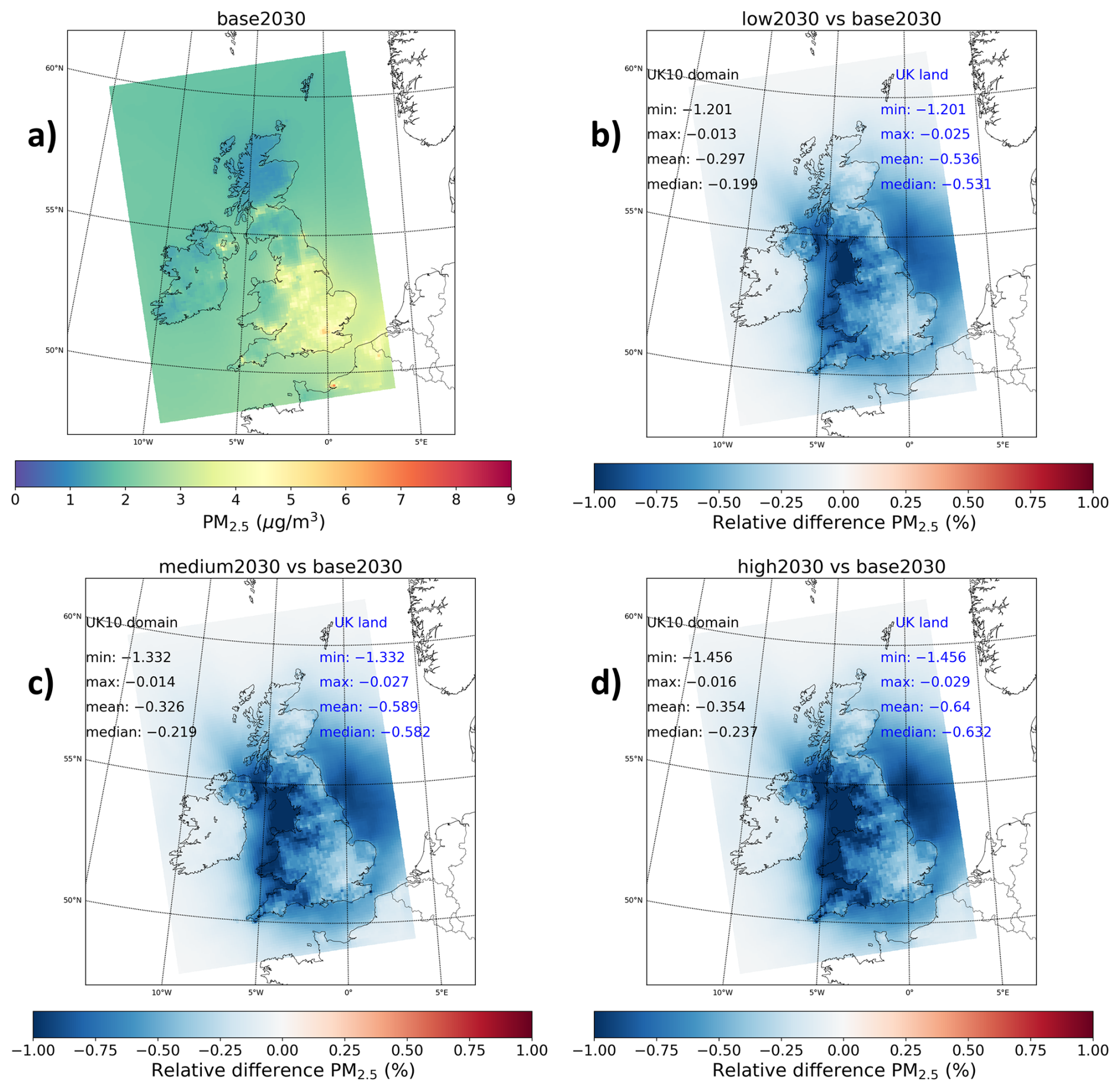
Figure 5 (a) Spatial distribution of annual mean PM_2.5 concentrations in µg m⁻³ calculated by CMAQ at 10 km resolution for the base2030 scenario. Relative difference of the same distribution with the low2030 (b), medium2030 (c), and high2030 (d) scenarios. The minimum, maximum, mean, and median relative difference values in the whole UK10 domain (in black) and for the UK land grid cells (blue) are provided. The relative difference is calculated as follows: ((scenario-base)$/$base) × 100 %.

Conversely, Ge et al. (2023) showed an important impact of the NH₃ emission reduction in PM_2.5 concentrations in the UK. The results in Ge et al. (2023) are not comparable with our study, since their analysis was based on a large decrease in the emissions – four times larger than our more ambitious mitigation (high2030) scenario. This difference in the assumption of the emission reduction has a crucial impact on the atmospheric chemical regime, therefore changing the influence of NH₃ in the SIA formation.

Moreover, the scenarios have focussed on mitigating NH₃ emissions, while targeting other secondary PM_2.5 precursors (NO_x and SO_x) can be required to effectively curb the PM_2.5 exposure (Marais et al., 2023; Pastorino et al., 2024). It is also worth noting that the impact of the mitigation measures, even limited, varies by months, showing a larger relative change in May–July (only up to −3.4 %) in the example of the high2030 scenario in Fig. S5. These months do not correspond to the maximum in the emitted NH₃ in the modelling, as shown in Fig. S1. This suggests also an impact of the atmospheric chemistry in the change in PM_2.5 concentrations.

The evaluation of CMAQ has shown a substantial negative bias in simulated PM_2.5 concentrations, affecting confidence in the absolute concentration levels. This also requires caution when interpreting the mitigation scenarios, because the simulated PM_2.5 responses are small. Since the baseline and scenario simulations use the same modelling framework, some systematic errors may partially cancel when scenario differences are calculated. These scenario results should therefore be interpreted as indicative of the direction and likely limited regional influence of NH₃-focussed mitigation on PM_2.5, rather than as precise quantitative estimates of change.

3.2 Local scale: dispersion near the farms

Regional modelling has been used to estimate the contribution of agricultural NH₃ to the formation of secondary PM_2.5 at a regional scale, whereas local-scale modelling has been used to investigate the dispersion of NH₃ and PM_2.5 closer to farms (within 10 km). This modelling approach differs from regional modelling, which incorporates atmospheric chemistry to estimate PM_2.5 from both primary emissions and secondary formation. While the local modelling considered a non-steady-state (reactive chemistry) option, secondary formation contributed less than 1 % of total PM_2.5 in the 10 km study area and was ultimately excluded from the analysis. However, both modelling approaches are linked since the regional modelled concentrations have been used to define the background concentrations.

As detailed in Sect. 2.1, low to high mitigation refers to mitigation uptake by a number of farms, but local modelling focuses on five specific farms, and variable uptake values are not relevant. Instead, consistent NH₃ impact values (percentage reduction) were adopted between regional and local modelling, with PM_2.5 impact values (percentage reductions) derived separately through best practice agricultural guidance (Santonja et al., 2017). Mitigation measures were assessed in the local modelling scenario to gauge the maximum potential benefit on pollutant concentrations in the local vicinity of farms.

Figure 6 represents study farms' contributions of NH₃ and primary PM_2.5 under existing farm operations (base2030), and the differences between the mitigation scenario and this reference. These farms were in different parts of the UK, as shown in Fig. 2. In the local modelling, the mitigation scenario incorporates all measures from the low2030, medium2030, and high2030 scenarios. While the regional modelling assumed progressively higher national uptake from low to high scenarios, the local modelling applied only those mitigation measures relevant to each specific farm. As a reminder, the mitigation measures for each farm are described in Table 2.

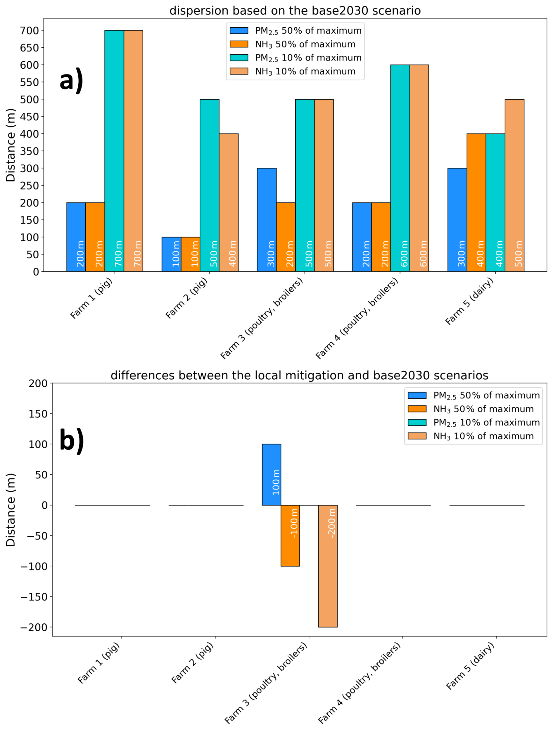
Figure 6 (a) Farms' contributions of NH₃ and primary PM_2.5 given as a distance in metres, with the concentration of 50 % or 10 % of maximum for the base2030 scenario (a), and the difference between the local mitigation scenario and the base2030 scenario (b).

Across the existing and mitigation scenarios, the greatest distance for concentrations of NH₃ and PM_2.5 to reach 10 % of the maximum is 700 m (Fig. 6a, b). The distance at which concentrations reach 10 % of the maximum varies depending on many local-scale dispersion parameters at the farm and meteorology, such as air flow release rate (m s⁻¹), temperature (°C), wind speed (m s⁻¹) and direction (°), and impact of building downwash. Indeed, such near-source concentrations in local modelling are highly sensitive to source geometry, release height, buoyancy, and initial momentum. Predictions beyond ∼ 100 m are less sensitive to source dimensions but can still depend strongly on efflux conditions and building effects (Stocker et al., 2015).

A total of 50 % of air pollutant concentrations from farm two are dispersed at a closer distance (100 m) than other farms due to an air flow rate of 5.1 m s⁻¹, whereas farms one, four, and five have a flow rate ranging between 7 and 11.5 m s⁻¹, which contributes to the plume grounding at a closer distance to farm two.

It is worth noting that the mitigation scenario solely impacts the distance of spread of the pollutants for farm three. Meanwhile, the distances where the 50 % of NH₃ and primary PM_2.5 concentrations are dispersed and the distances where 10 % of their maximum concentrations are found are identical for the other farms (Fig. 6b). However, as illustrated in Fig. S6, farm three did not contribute to PM_2.5, and the NH₃ concentration remained highly localized around the farm.

The highest NH₃ concentrations occur in the vicinity of the emission sources, as shown in Fig. S6 for farm three. This is driven by the low release heights (< 6 m) typical of agricultural emissions and, in several cases, by the enhancement of near-field concentrations due to building-induced flow effects. Concentrations decline rapidly with distance, and beyond very short distances the influence of farm-level emissions diminishes sharply.

The difference in concentrations between the mitigation and base2030 scenarios are presented in Table 3 for maximum concentration in a 10 km² area and maximum concentration for sensitive receptors. Table 3 shows that within 1 km of farms included in this study, there can be reductions of between 25 % and 80 % in total NH₃ concentrations, and between 4 % and 60 % reductions in PM_2.5.

Table 3 Per cent difference in concentrations between base2030 and mitigation scenarios.

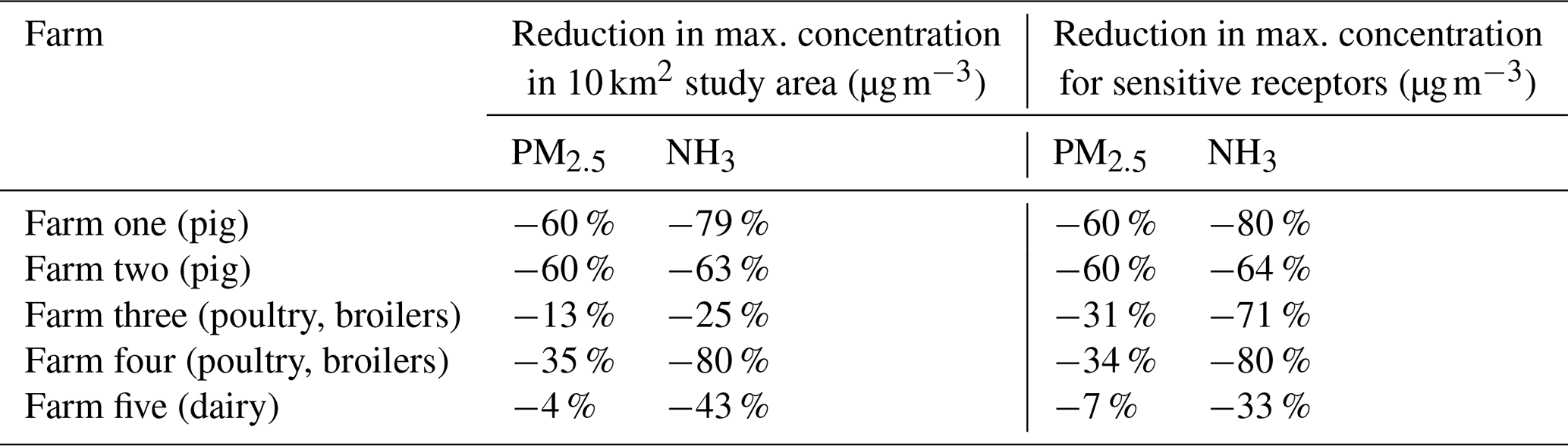
The biggest reductions in pollutant concentrations occur at farms one and two, which are pig farms. The abatement measure with the biggest benefit is an acid scrubber used to reduce emissions from housing and, as shown in Table 2, is estimated to achieve an 80 % reduction in NH₃ and a 60 % reduction in PM_2.5 emissions.

The only other relevant mitigation measure included at farms one and two would be to provide a cover over open manure and/or slurry lagoons; however, this has a smaller 60 % reduction of only NH₃ emissions and will have a smaller impact on NH₃ concentrations than the acid scrubber. While acid scrubbers and manure/slurry covers are included in the modelling of estimated concentration, the biggest will come from acid scrubbers.

4 Discussion

The design of the emission scenarios was based on the views of farmers, advisers, academics, and representatives from relevant sectors, capturing diverse perspectives and making the uptake scenarios grounded in real-world practices and challenges. This approach also considered the actual barriers and incentives that farmers experience, leading to realistic projections of mitigation measure uptake. Using multiple engagement tools (online surveys, focus groups, and one-on-one interviews) also enabled the gathering of in-depth, well-rounded data, providing a nuanced understanding of the factors influencing uptake. However, it is worth noting that the future uptake projections did not account for potential changes in legislation, which could significantly impact the adoption of mitigation measures. This limits the ability to predict uptake under different regulatory environments. Moreover, the method has not differentiated uptake scenarios between different parts of the UK due to a lack of data, potentially overlooking regional variations in farming practices, environmental conditions, or economic incentives. The study has also relied on subjective feedback, i.e. participants' perception and understanding, which can vary widely between individuals or groups. This can introduce bias in determining which measures are positively or negatively received, potentially affecting the estimated uptake rates.

Although CMAQ is state of the art and widely used in scientific research and policy development, the model also has uncertainties. The analysis presented in this study relies on the accuracy of the simulation, which is subject to any uncertainties in the model's specific parameterization of atmospheric processes, as well as uncertainties in the emission inventory and meteorology input. It has been shown that CMAQ does not perfectly model the interactions between NH₃ emissions. In addition, the local processes cause the majority of NH₃ to be dispersed near the studied farms, as highlighted by ADMS results. The ADMS results showed a steep decline in farm-scale NH₃ and primary PM_2.5 concentrations, with concentrations decreasing by around 90 % within 700 m of the studied farms. This indicates strong near-source concentration gradients and highlights the importance of local exposure close to farms.

The limited impact of the mitigation measures at a regional scale, which mainly target the NH₃ emissions, on PM_2.5 concentrations can be due to an NH₃-rich atmosphere in the UK and highlights the fact that other precursors of these PM_2.5 emissions and the primary PM_2.5 emissions need to be tackled. This confirms the findings of Pan et al. (2024) arguing for more collocated aerosol and precursor observations for better characterization of SIA formation. This also emphasizes that exposure to secondary PM_2.5 near farms also needs to be investigated, although most air quality studies focus on total PM_2.5 concentrations.

Further work is recommended to assess how mitigation measures can affect primary and secondary PM_2.5 at relevant human exposure locations within 1–10 km of farms, given that national exposure weighting emphasizes locations where most primary pollution has already dispersed.

Limitations of the local modelling include uncertainties related to the model parameterization, emission measurement data, and the associated farm activity data. A targeted local-scale modelling study can be developed to evaluate how variations in parameters such as emission factors, turbulence, and deposition velocities influence pollutant dispersion in the vicinity of the farms. The project measurement study (Leonard and Wiltshire, 2025) should be referenced for the full suite of limitations associated with project measurement data; however, the main aspects that affect emission rates developed for local modelling includes the representativeness of measurement location for entire housing unit, and measurements did not span an entire animal cycle at farms one, two, and five. Regarding the representativeness of measurements, at farms three and five, housing air was sampled with a multiplexer, a device that samples air from multiple locations, whereas measurements at other farms only sampled air from one location. Consequently, a limitation of emission rates used in modelling is the assumption that emission rates are representative for the entire animal housing unit. Measurement data did not span entire animal life cycles at farms one, two, and five, and therefore the project measurement data and housing emissions rates are limited in how representative they are of each animal life cycle. Further to this, farms one, two, and five did not record animals in each housing unit for each day of the measurement period and over the animal life cycle; instead, assumptions were made on the total number of animals apportioned to each housing unit. Consequently, there is uncertainty regarding animal numbers in each housing unit and the extrapolations made for the annual animal places at farms one, two, and five. While farms two and three had measurements for the entire animal cycle, like farms one and two, measured fan flow rates were not available during the measurement period and ventilation manufacturer's records were used to develop air flow rates. While there are limitations in data used, replacing emission and flow rate assumptions is unlikely to alter the fact that the majority of pollution is grounded in the near-field (< several kilometres) of farms (e.g. AFBI, 2025), since agricultural sources are emitted from lower heights (< 6 m) and have low air flow rates relative to other sources such as engine exhausts.

5 Conclusions and perspectives

This study highlights the complex interactions between NH₃ emissions from farming activities and PM_2.5 formation in the UK, with a focus on the dairy, pig, and poultry sectors. Using both the CMAQ model for regional-scale analysis and ADMS for local-scale dispersion, this work has evaluated the impact of mitigation measures under various uptake scenarios on reducing emissions, especially on NH₃. Although emission reductions, particularly in NH₃, were predicted under a high-uptake scenario, these changes did not translate into significant reductions in regional-scale PM_2.5 concentrations, with a maximum decrease of only 1.5 %. This outcome is attributed to the NH₃-rich atmosphere, which diminishes the effect of NH₃ reductions on PM_2.5 mitigation.

The findings also reveal discrepancies between CMAQ model concentrations and ground-based measurements. Although this bias aligns with findings in the literature, particularly when no emission corrections or post-processing adjustments to modelled concentrations are applied, this suggests that key atmospheric processes influencing PM_2.5 formation may not be fully represented in the model, leading to an underestimation of PM_2.5 concentrations by approximately 50 %. ADMS results further show that NH₃ is rapidly dispersed near the farms, indicating a limited role of these emissions in the formation of PM_2.5 locally. The study has emphasized the need for integrated modelling approaches and better characterization of SIA formation, as well as the importance of addressing the primary PM_2.5 and other PM_2.5 precursors beyond NH₃ to achieve effective air quality improvements.

Overall, this suggested limited impact on potential NH₃-focussed mitigation strategies on PM_2.5 concentrations underscores the necessity of exploring additional emission control measures targeting other precursors and primary PM_2.5 emissions from the farming sector. Indeed, further work is recommended to review the national benefit of mitigation on primary PM_2.5 emissions; however, benefits of mitigation are likely to be localized on PM_2.5, as demonstrated by ADMS modelling. Future research should also focus on primary and secondary PM_2.5 exposure separately near farms, as current air quality studies predominantly assess total PM_2.5 concentrations, and further work is required to understand the impact of secondary PM_2.5 on health. This work advocates for a more holistic approach to modelling and mitigation to better inform policies aimed at improving air quality in agricultural regions.

The study has looked at regional exposure to PM_2.5 from agricultural sources in CMAQ, whereas ADMS has shown that the majority (90 %) of emissions are dispersed within 700 m of farms. As the UK population is concentrated in urban areas, a substantial distance from farms, further work could explore the health benefit of mitigation on communities in the local vicinity of farms (from 1 to 10 km). To evaluate the potential impact of these emissions on rural populations, one approach would be to map population distribution around agricultural holdings. This would help to estimate the number of individuals likely to be exposed to such emissions. Although the study primarily addresses annual estimates, further investigations at finer temporal resolutions (e.g. daily, monthly) could yield deeper insights into exposure impacts. To strengthen our understanding of near-field NH₃ impacts, future work would benefit from expanded measurement campaigns across a wider range of farm types, not only increasing the number of monitoring sites but also ensuring a balanced representation across key sectors such as poultry, pig, and dairy systems.

Finally, the simulations were performed using meteorological fields from a single year (2019), and future work could incorporate multi-year or climate-perturbed meteorological data sets to better characterize the influence of meteorological variability on agricultural PM_2.5 formation.

Appendix A

Table A1 summarizes the measures and the uptake rates for each of the three scenarios for the regional modelling. These values are additional to the uptake of measures already included in emissions from NAEI.

The uptake scenarios were developed through stakeholder engagement with farmers and stakeholders (i.e. farm advisers, academics, and farmer representatives). Each scenario includes all 20 mitigation measures, however with varying percentages of uptake.

Table A1 A summary of the measures and uptake rates used in each of the three scenarios modelled for this study.

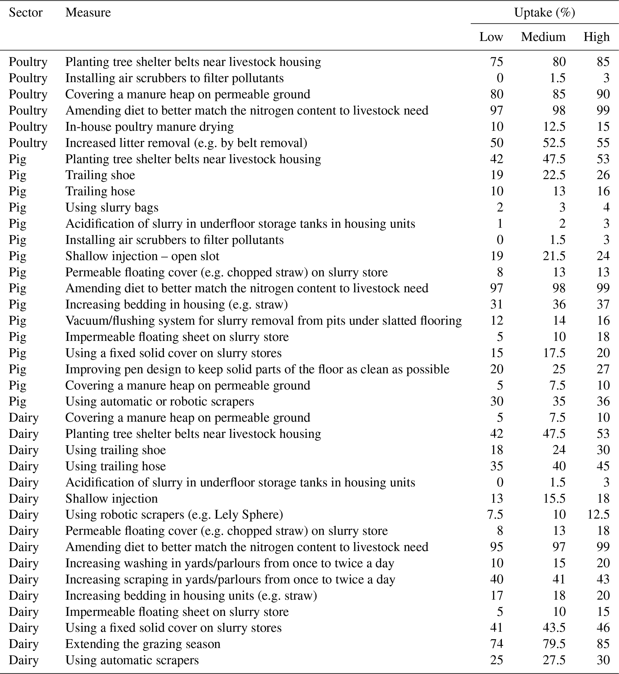
The uptake rates were unique to each mitigation measure in each sector and were reflective of feedback received through engagement activities. The engagement activities included an online survey, focus groups, and one-on-one interviews with participants from the dairy, pig, and poultry sectors, and those in other sectors that utilize manure or slurry. A total of 161 people took part in the activities. Full results and methodology are detailed in Jenkins and Wiltshire (2025).

Discussions in these activities were centred around understanding the current level of uptake, and the benefits and barriers associated with the mitigation measures, to determine a potential future uptake. If a mitigation measure was received positively, it was estimated to have a higher uptake compared to measures that were received negatively by participants. This was determined in the final level of uptake for each scenario. The future uptake did not take into account any potential changes to legislation that may have an impact, as this information is not known; additionally, there were no different uptakes for each part of the UK due to a lack of data.

Appendix B

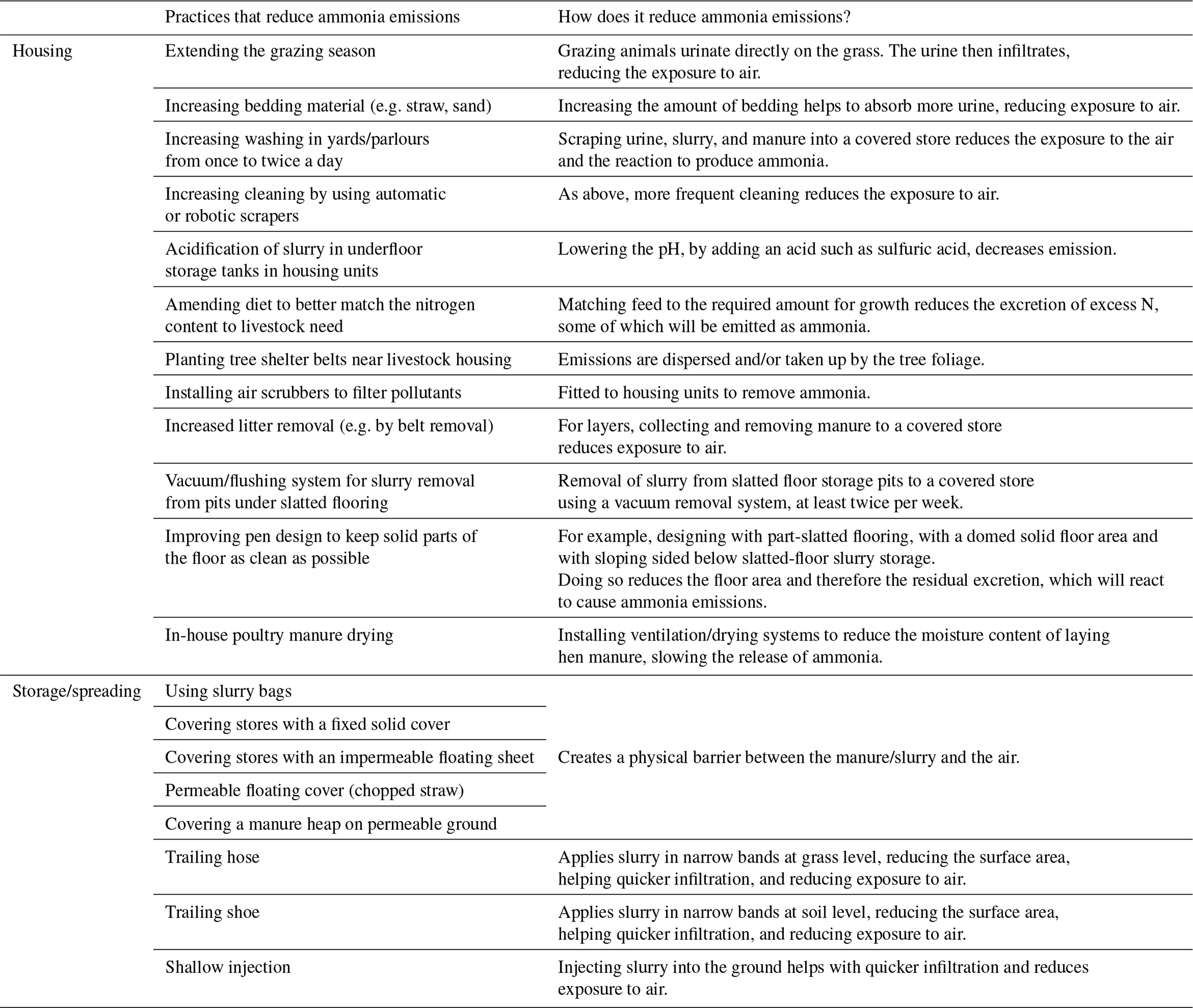
Table B1 presents the practices that reduce ammonia emissions that were modelled in this study, along with a brief description on how it reduces ammonia.

Table B1 Practices that reduce ammonia emissions, with a short description of how they reduce emissions.

Appendix C

Statistics used for the evaluation of the air quality simulation with CMAQ. In the following notations, M and O refer, respectively, to the model and the observation data. N is the number of the observation data set.

•  

  Pearson relation coefficient (r). The ideal score of these parameters is 1. It is a unitless variable.

•  

  Mean bias (MB). The ideal score of this parameter is 0. The unit of this variable is the pollutant concentration (µg m⁻³). The MB provides information about the absolute bias of the model, with negative values indicating underestimation and positive values indicating overestimation by the model.

  $$\begin{array}{}\text{(C1)}& \text{MB}={\displaystyle \frac{{\sum }_{i=\mathrm{1}}^N\left(M_i-O_i\right)}{N}}\end{array}$$
•  

  Normalized mean bias (NMB). The ideal score of this parameter is 0, and the unit of the variable is in per cent. The NMB represents the model bias relative to the reference.

  $$\begin{array}{}\text{(C2)}& \text{NMB}={\displaystyle \frac{{\sum }_{i=\mathrm{1}}^N\left(M_i-O_i\right)}{{\sum }_{i=\mathrm{1}}^N{O}_i}}\times \mathrm{100}\mathit{\%}\end{array}$$
•  

  Root mean square error (RMSE). The ideal score of this parameter is 0. The unit of this variable is the as the pollutant concentration (µg m⁻³). The RMSE considers error compensation due to opposite sign differences and encapsulates the average error produced by the model.

  $$\begin{array}{}\text{(C3)}& \text{RMSE}=\sqrt{{\displaystyle \frac{{\sum }_{i=\mathrm{1}}^N{\left(M_i-O_i\right)}^{\mathrm{2}}}{N}}}\end{array}$$
•  

  Mean relative error (MRE). The ideal score of this parameter is 0. The MRE is the mean ratio of difference between the model values and the observations, on the observations. This variable is unitless.

  $$\begin{array}{}\text{(C4)}& \text{MRE}={\displaystyle \frac{\mathrm{1}}{N}}{\sum }_{i=\mathrm{1}}^N{\displaystyle \frac{M_i-O_i}{O_i}}\end{array}$$
•  

  Index of agreement (IOA). The agreement value of 1 indicates a perfect match, and 0 indicates no agreement at all. It is a unitless variable.

  $$\begin{array}{}\text{(C5)}& \text{IOA}=\mathrm{1}-{\displaystyle \frac{{\sum }_{i=\mathrm{1}}^N{\left(M_i-O_i\right)}^{\mathrm{2}}}{{\sum }_{i=\mathrm{1}}^N(\left|M_i-\stackrel{\mathrm{‾}}{O}\right|+\left|O_i-\stackrel{\mathrm{‾}}{O}\right|{)}^{\mathrm{2}}}}\end{array}$$