Numerical study of the collection of aerosol particles by falling deformable drops

The free fall of a drop through gas loaded with solid particles gives rise to multiple physical interactions, which remain poorly documented, especially when the drop is no longer spherical. In particular, no model predicts the particle collection efficiency for drops undergoing deformations or oscillations. This study aims to contribute to this effort by investigating numerically the dynamics of water drops freely falling in air laden with dispersed solid particles for drop Reynolds and Weber numbers such that the drops do (or do not) deform or oscillate (e.g., Re=30, 70, 500, and 876). A Eulerian–Lagrangian framework is adopted. The drop internal and external flows are simulated with direct numerical simulation (DNS), and the dynamics of the liquid–gas interface are tracked using a combination of the volume of fluid (VOF) and level set methods; this approach predicts the interface dynamics in line with experimental data. The trajectories of solid particles are simulated using Lagrangian tracking and taking into account drag, gravity, and Brownian motion. For spherical drops with Reynolds numbers below 200, our methodology replicates previous results. In the presence of oscillations and/or deformations, the flow parameters of the two continuous phases are correctly predicted. The particle collection efficiency also follows the experimental trend, but the values differ significantly from measurements found in the literature. We therefore propose certain areas of improvement with the goal of obtaining better fits to the available experimental data.

1 Introduction

In many industrial and environmental contexts, the air is loaded with aerosol pollutants, such as dust, smoke, pathogens, or radioactive particles. Workers thus frequently face exposure to air polluted with aerosol particles, which can cause serious health risks, leading to respiratory problems and other adverse health effects. During nuclear accidents, a significant amount of radioactive materials can also be released into the environment in the form of aerosol particles that can ultimately get inhaled, causing harmful health effects. Reducing particulate emissions and concentration in the air is a central issue for which effective control methods are needed. In these contexts, the washout or scrubbing of aerosol particles by free-falling drops is a standard process to decrease the concentration of airborne aerosol particles (Greenfield, 1957).

At the scale of a single drop, the effectiveness of this process, as per the primary purpose of this study, is modeled with a micro-physical parameter called collection efficiency, E. It is defined as the ratio between the number of aerosol particles collected by a falling drop and the total number of particles in the volume swept up by the drop. In the literature, Slinn (1977) was the first to establish models to calculate this efficiency using particle flow balances, assuming potential flows around the drop and a decoupling of the collection mechanisms. The limitations of this approach were partially overcome in later work. Grover and Pruppacher (1977) were the first to theoretically establish collection efficiencies based on Lagrangian tracking of particles around drops by calculating direct numerical simulation (DNS) flows for spherical drops, with Reynolds numbers below 200, taking into account drag and electric forces on aerosols. However, they did not consider Brownian motion in their Lagrangian tracking despite its influence on sub-micron particles. More recently Minier and Peirano (2001) integrated analytically the approach of Langevin (1908) for Brownian motion of aerosols. Thanks to this approach, Cherrier et al. (2016) added Brownian motion to the Grover and Pruppacher (1977) approach, and their results were validated with efficiency measurements performed in the laboratory by Dépée et al. (2021).

Despite this conceptual unification, a major scientific challenge remains. These approaches require an accurate simulation of the flow around the drop. However, drops with a Reynolds number above 500 oscillate at high frequencies and deform progressively (Szakáll et al., 2010). For such a task, the methods deployed by Cherrier et al. (2016) and Dépée et al. (2021) – relying on a fixed geometry – are no longer valid. Our work proposes an alternative method to extend computations to include Reynolds numbers above 200. The liquid–gas interface dynamics are now modeled using a hybrid volume of fluid (VOF)–level set method (CLSVOF, here in a momentum-conserving variant published by Vaudor et al., 2017) coupled to a DNS solver applied to both continuous phases. In contrast, the motion of the discrete aerosol phase is modeled in the same Lagrangian framework as that introduced by Cherrier et al. (2016), accounting for the drag force and Brownian motion.

To validate this approach, tests are first carried out to ensure that the model predictions stay within the state of the art. First, free-falling water drops of Reynolds numbers 30 and 70 exhibiting no oscillation or deformation are simulated as they interact with aerosol particles with aerodynamic diameters ranging from 2 nm to 20 µm. The drop-settling velocities and velocity fields inside and outside the drop are compared with results from the literature (Beard, 1976; Cherrier et al., 2016). Similarly, the aerosol collection efficiencies are compared with results from the literature (Cherrier et al., 2016). Tests of the independence of the results concerning the numerical resolution parameters are carried out (mesh convergence and interpolation order). Secondly, simulations are performed for flow regimes with drop oscillation and deformation, for which – to our knowledge – no simulation results of aerosol particle collection efficiency are available in the literature. We chose the case of 1.39 and 2 mm diameter water drops falling freely under ground-based atmospheric conditions (drop Reynolds numbers of 500 and 876), for which experimental validation data are available. For these situations, the simulation results for the continuous phases are hence validated by comparison with experimental results, as done by Ren et al. (2020) (terminal fall velocity, mean drop axis ratio, and characteristic oscillation frequencies, Beard, 1976; Szakáll et al., 2010). For the aerosol phase, the collection efficiencies are compared with experimental results from the literature (Quérel et al., 2014; Lai et al., 1978), considering the poly-dispersion of the aerosol sizes involved.

This approach to evaluate the proposed method is described in Sects. 5 and 6 of the paper after a presentation of the physical modeling of the system under consideration and the numerical methods used for its approximate resolution.

2 Physical model

Our simulations consider a free-falling drop in quiescent air at atmospheric pressure ($P=P_{\text{atm}}=\mathrm{101}$ kPa, T=293.15 K).

2.1 Continuous phase

The motion of the continuous phases, consisting of both an inner flow (water) and an outer flow (air), is simulated by solving numerically the same Navier–Stokes equations, assuming incompressibility:

$$\begin{array}{}\text{(1)}& \left\{\begin{array}{l}\frac{\partial \mathit{\rho }\left(\mathit{\psi }\right)\mathit{U}}{\partial t}+\mathbf{\nabla }\cdot \left(\mathit{\rho }\right(\mathit{\psi })\mathit{U}\otimes \mathit{U})\\ =-\mathbf{\nabla }p+\mathbf{\nabla }\cdot \left(\mathrm{2}\mathit{\mu }\right(\mathit{\psi }\left)D\right)+\mathit{\rho }\left(\mathit{\psi }\right)\mathit{g}+\mathit{\sigma }\mathit{\kappa }\left(\mathit{\psi }\right)\mathit{\delta }\left(\mathit{\psi }\right)\mathit{n}\\ \mathbf{\nabla }\cdot \mathit{U}=\mathrm{0}\end{array}\right.,\end{array}$$

where ρ, U, and p are the density, velocity, and pressure, respectively; $D=\frac{\mathrm{1}}{\mathrm{2}}(\mathbf{\nabla }\mathit{U}+\mathbf{\nabla }{\mathit{U}}^T)$ is the strain rate tensor; μ is the dynamic viscosity; and ρ(ψ)g denotes the gravity forces. The surface tension forces are considered to be expressed by σκ(ψ)δ(ψ)n, with σ being the surface tension, κ(ψ) being the local curvature of the interface, and δ(ψ) being the Dirac function. ψ is the phase indicator which is used to reconstruct the interface at each time step; it can be either the level set function (ϕ) or the VOF function (C) depending on the quantity (ρ, μ, etc.) to be determined (Vaudor et al., 2017).

In the present simulations, the absolute velocities of both fluids are calculated in the drop reference frame. The convective velocity in the equations must, therefore, be U−U_d, where U_d is the instantaneous velocity of the drop calculated at each time step. The equations are hence transformed as follows:

$$\begin{array}{}\text{(2)}& \begin{array}{rl}& {\displaystyle \frac{\partial \mathit{\rho }\left(\mathit{\psi }\right)\mathit{U}}{\partial t}}+\mathbf{\nabla }\cdot \left(\mathit{\rho }\right(\mathit{\psi }\left)\right(\mathit{U}-{\mathit{U}}_{\mathrm{d}})\otimes \mathit{U})\\ & =-\mathbf{\nabla }p+\mathbf{\nabla }\cdot \left(\mathrm{2}\mathit{\mu }\right(\mathit{\psi }\left)D\right)+\mathit{\rho }\left(\mathit{\psi }\right)\mathit{g}+\mathit{\sigma }\mathit{\kappa }\left(\mathit{\psi }\right)\mathit{\delta }\left(\mathit{\psi }\right)\mathit{n}.\end{array}\end{array}$$

The numerical resolution of Eq. (1) requires the determination of a function ψ. An additional equation, Eq. (4), is solved concurrently to achieve this. This equation specifically deals with the transport and evolution of the interface by the flow between the different phases (in our case, the boundary between air and water) within the computational domain. The parameter ψ can represent either the interface distance function level set (ϕ) or VOF (C) functions, which are coupled as described by Sussman and Puckett (2000). The interface is defined by zero level set surface/curve (ϕ=0 in 3D/2D, respectively), and the VOF function represents the volume fraction of liquid in a cell:

$$\begin{array}{}\text{(3)}& C={\displaystyle \frac{\mathrm{1}}{V}}\underset{V}{\int }H\left(\mathit{\varphi }\right)\mathrm{d}V,\end{array}$$

where H is the Heaviside function, equal to 1 in the liquid and 0 in the air. Advection of both functions is achieved by solving the following equation:

$$\begin{array}{}\text{(4)}& {\displaystyle \frac{\partial \mathit{\psi }}{\partial t}}+\mathrm{\nabla }\cdot (\mathit{U}-{\mathit{U}}_{\mathrm{d}})\mathit{\psi }=\mathrm{0},\end{array}$$

which is coupled with an additional equation to preserve the distance function property of the level set ($\Vert \mathrm{\nabla }\mathrm{\Phi }\Vert =\mathrm{1}$) (Sussman et al., 1994; Min and Gibou, 2007). Physical parameters are computed with the help of the VOF function, while geometrical characteristics are computed with either the level set function or the VOF function.

$$\begin{array}{c}{\displaystyle }\mathit{\rho }\left(C\right)=C{\mathit{\rho }}_{\mathrm{l}}+(\mathrm{1}-C){\mathit{\rho }}_{\mathrm{g}}\\ {\displaystyle }\mathit{\mu }\left(C\right)=C{\mathit{\mu }}_{\mathrm{l}}+(\mathrm{1}-C){\mathit{\mu }}_{\mathrm{g}}\\ {\displaystyle }\mathit{n}={\displaystyle \frac{\mathrm{\nabla }\mathit{\varphi }}{\left|\mathrm{\nabla }\mathit{\varphi }\right|}}\\ {\displaystyle }\mathit{\kappa }\left(\mathit{\varphi }\right)=\mathrm{\nabla }.\mathit{n}\\ {\displaystyle }\mathit{\delta }\left(\mathit{\psi }\right)\mathit{n}=\mathrm{\nabla }C\end{array}$$

2.2 The discrete phase

A Lagrangian approach is used to model the transport of aerosol particles by the continuous phases. Each aerosol particle is treated as a discrete entity, and its motion is governed by drag forces and Brownian motion. The state vector of each particle is ${\mathit{Z}}_{\mathrm{p}}\left(t\right)=\mathit{\left\{}{\mathit{x}}_{\mathrm{p}}\right(t),{\mathit{U}}_{\mathrm{p}}(t\left)\mathit{\right\}}$, where x_p(t) is the instantaneous position of the particle in the flow, and U_p(t) is its velocity. Smaller particles (sizes below 1 µm) are sensitive to Brownian effects, while larger ones follow their inertia. The equations of motion retained correspond to the Langevin equations:

$$\begin{array}{}\text{(5)}& \left\{\begin{array}{l}\mathrm{d}{\mathit{x}}_{\mathrm{p}}=\left({\mathit{U}}_{\mathrm{p}}\left(t\right)-{\mathit{U}}_{\mathrm{d}}\left(t\right)\right)\mathrm{d}t\\ \mathrm{d}{\mathit{U}}_{\mathrm{p}}={\displaystyle \frac{{\mathit{U}}_{\mathrm{f}}\left(t\right)-{\mathit{U}}_{\mathrm{p}}\left(t\right)}{{\mathit{\tau }}_{\mathrm{p}}}}\mathrm{d}t+Bd\mathit{W}\left(t\right)\end{array}\right.,\end{array}$$

where U_f is the fluid velocity at the particle's position, and τ_p is the relaxation time of the particle (taking into account the Cunningham correction for rarefaction effect). The last term of the equation represents the Brownian effects, with dW being the increment of the Wiener process and B being the diffusion coefficient (Minier and Peirano, 2001). Effectively, this represents a one-way coupled system which is justified at the volume fraction considered in our work, as shown in Elgobashi (1984).

2.3 Capture criteria

In our modeling framework, the particles are considered to be “collected” as long as they enter into geometrical contact with the drop, which is in line with theoretical predictions (Wang et al., 2015). In order to determine if the particles enter into contact with the drop during the Lagrangian tracking, the level set value at the particle location (ϕ_p) is compared at each time step. Hence, the capture condition can be expressed as follows:

$$\begin{array}{}\text{(6)}& {\mathit{\varphi }}_{\mathrm{p}}+r_{\mathrm{p}}\ge \mathrm{0},\end{array}$$

which – considering the fact that ϕ is (by choice) set as negative outside of the droplet – means simply that its surface contacts the particle (which is closer to it than its radius r_p). Once that happens, the trajectory calculation for the particle is terminated, and the particle is considered to be captured by the falling drop. This formulation accounts for the varying shape and size of the drop throughout its deformation process.

2.4 Collection efficiency

For each particle diameter, the collection efficiency E is defined as the ratio between the particle number flow rate collected by the drop during its fall and the particle number flow rate in the cross-section of the drop. During a single Lagrangian particle release, N_inj particles are injected into the upstream flow of the drop. These particles are injected homogeneously inside a “virtual disk” placed upstream of the drop (as detailed in Sect. 4.3); afterwards, E is computed from the following:

$$\begin{array}{}\text{(7)}& E(d_{\mathrm{d}},d_{\mathrm{p}})={\displaystyle \frac{N_{\text{capt}}\left(d_{\mathrm{p}}\right)}{N_{\text{inj}}\left(d_{\mathrm{p}}\right)}},\end{array}$$

where N_capt is the number of particles captured by the drop, while d_d and d_p are the drop and particle diameter, respectively.

3 Numerical methods

3.1 Continuous phases

The simulations in this study are conducted using an in-home academic code, ARCHER (Academic Research Code for Hydrodynamic Equations Resolution), originally created by a team led by Alain Berlemont (Tanguy and Berlemont, 2005; Ménard et al., 2007; Vaudor et al., 2017). Its aim is to carry out DNS simulations for multiphase flow simulations with a range of interface representations (Aniszewski et al., 2014) and a multitude of physical phenomena (Duret et al., 2013). Many implementation details can be found in Vaudor et al. (2017). In Archer, the temporal integration is carried out using either the Euler or the second-order Runge–Kutta scheme. Volume of fluid (VOF) and level set interface-tracking functions are first advected explicitly to allow the calculation of physical parameters at time n+1. Then a projection method is used by introducing an intermediate velocity U^* to solve the momentum equation without the pressure term (Eq. 8) and the velocity Uⁿ⁺¹ and pressure correction (Eq. 9).

$$\begin{array}{}\text{(8)}& {\displaystyle }\begin{array}{rl}{\mathit{U}}^{*}& ={\displaystyle \frac{{\mathit{\rho }}^n{\mathit{U}}^n}{{\mathit{\rho }}^{n+\mathrm{1}}}}+{\displaystyle \frac{\mathrm{\Delta }t}{{\mathit{\rho }}^{n+\mathrm{1}}}}(\mathbf{\nabla }\cdot (\mathit{\rho }\left(C\right)\mathit{U}\otimes \mathit{U})+\mathbf{\nabla }\cdot (\mathrm{2}\mathit{\mu }\left(C\right)D){)}^n\\ & +{\displaystyle \frac{\mathrm{\Delta }t}{{\mathit{\rho }}^{n+\mathrm{1}}}}\left(\right(\mathit{\rho }\left(C\right)-{\mathit{\rho }}_{\mathrm{g}})\mathit{g}+\mathit{\sigma }\mathit{\kappa }(\mathit{\varphi }=\mathrm{0}\left)\mathit{\delta }\right(\mathit{\psi })\mathit{n}{)}^{n+\mathrm{1}}\end{array}\text{(9)}& {\displaystyle }{\mathit{U}}^{n+\mathrm{1}}={\mathit{U}}^{*}-\mathrm{\Delta }t\left({\displaystyle \frac{\mathbf{\nabla }{p}^{n+\mathrm{1}}}{{\mathit{\rho }}^{n+\mathrm{1}}}}\right)\end{array}$$

The discretization of the convective term, the weighted essentially non-oscillatory (WENO) scheme, is employed based on the conservative discretization described by Vaudor et al. (2017). The standard continuum surface force (CSF) method (Popinet, 2018) is used to handle the surface tension term, where δ(ψ)n is approximated by ∇C (see also Aniszewski, 2016).

Applying the divergence operator to Eq. (9), with the help of the continuity equation $\mathbf{\nabla }.{\mathit{U}}^{n+\mathrm{1}}=\mathrm{0}$, allows us to write the following Poisson equation, Eq. (10), which yields the pressure field. The velocity field Uⁿ⁺¹ is deduced with Eq. (9).

$$\begin{array}{}\text{(10)}& \mathbf{\nabla }.\left({\displaystyle \frac{\mathbf{\nabla }{p}^{n+\mathrm{1}}}{{\mathit{\rho }}^{n+\mathrm{1}}}}\right)={\displaystyle \frac{\mathbf{\nabla }\cdot {\mathit{U}}^{*}}{\mathrm{\Delta }t}}\end{array}$$

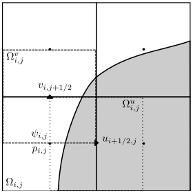
The velocity field and the interface distance values (given by the level set ϕ) are discretized on a uniform Cartesian mesh ($\mathrm{\Delta }x=\mathrm{\Delta }y=\mathrm{\Delta }z$). In our program, the Marker and Cell (Welch et al., 1965) method is used: scalar quantities (VOF, distance function, pressure) are located at mesh centers, while vector quantities are positioned on the faces, resulting in a staggered mesh (Fig. 1).

Figure 1 Representation of control volumes Ω on a staggered grid.

3.2 Discrete phase

A discretized version of Eq. (5), proposed by Mohaupt et al. (2011), is used to track the trajectories of the particles. The discretized version involves numerical approximation methods to solve the equations and to calculate the particle positions and velocities at each time step:

$$\begin{array}{}\text{(11)}& \left\{\begin{array}{l}{\mathit{x}}_{\mathrm{p}}(t+\mathrm{\Delta }t)={\mathit{x}}_{\mathrm{p}}\left(t\right)+\left({\mathit{U}}_{\mathrm{p}}\right(t)-{\mathit{U}}_{\mathrm{d}}(t\left)\right){\mathit{\tau }}_{\mathrm{p}}(\mathrm{1}-e^{-\frac{\mathrm{\Delta }t}{{\mathit{\tau }}_{\mathrm{p}}}})\\ +{\mathit{U}}_{\mathrm{f}}(\mathrm{\Delta }t-{\mathit{\tau }}_{\mathrm{p}}(\mathrm{1}-e^{-\frac{{\mathrm{\Delta }}_{\mathrm{p}}}{{\mathit{\tau }}_{\mathrm{p}}}}\left)\right)\\ +B{\mathit{\tau }}_{\mathrm{p}}\sqrt{\mathrm{\Delta }t-\mathrm{2}{\mathit{\tau }}_{\mathrm{p}}\frac{\left(\mathrm{1}-e^{-\frac{\mathrm{\Delta }t}{{\mathit{\tau }}_{\mathrm{p}}}}\right)}{\left(\mathrm{1}+e^{-\frac{\mathrm{\Delta }t}{{\mathit{\tau }}_{\mathrm{p}}}}\right)}}{\mathit{\xi }}_x\\ +B{\mathit{\tau }}_{\mathrm{p}}^{\mathrm{2}}\frac{{\left(\mathrm{1}-e^{-\frac{\mathrm{\Delta }t}{{\mathit{\tau }}_{\mathrm{p}}}}\right)}^{\mathrm{2}}}{\sqrt{\mathrm{2}{\mathit{\tau }}_{\mathrm{p}}(\mathrm{1}-e^{-\mathrm{2}\frac{\mathrm{\Delta }t}{{\mathit{\tau }}_{\mathrm{p}}}})}}{\mathit{\xi }}_v\\ {\mathit{U}}_{\mathrm{p}}(t+\mathrm{\Delta }t)={\mathit{U}}_{\mathrm{p}}\left(t\right)e^{-\frac{\mathrm{\Delta }t}{{\mathit{\tau }}_{\mathrm{p}}}}+{\mathit{U}}_{\mathrm{f}}(\mathrm{1}-e^{-\frac{\mathrm{\Delta }t}{{\mathit{\tau }}_{\mathrm{p}}}})\\ +B\sqrt{\frac{{\mathit{\tau }}_{\mathrm{p}}}{\mathrm{2}}(\mathrm{1}-e^{-\mathrm{2}\frac{\mathrm{\Delta }t}{{\mathit{\tau }}_{\mathrm{p}}}})}{\mathit{\xi }}_v\end{array}\right.,\end{array}$$

with ξ_x and ξ_v representing independent random variable vectors sampled in a normal distribution. In Eq. (11), B is a coefficient relating the diffusion properties of the aerosol particle due to Brownian motion:

$$\begin{array}{}\text{(12)}& B^{\mathrm{2}}={\displaystyle \frac{\mathrm{2}{k}_{\mathrm{b}}\mathit{\theta }}{m_{\mathrm{p}}{\mathit{\tau }}_{\mathrm{p}}}},\end{array}$$

with θ being the temperature, k_b being the Boltzmann constant, and m_p being the mass of the particle. For Re≪1, τ_p can be defined as follows:

$$\begin{array}{}\text{(13)}& {\mathit{\tau }}_{\mathrm{p}}={\displaystyle \frac{{\mathit{\rho }}_{\mathrm{p}}{d}_{\mathrm{p}}^{\mathrm{2}}}{\mathrm{18}{\mathit{\mu }}_{\mathrm{f}}}}\mathit{\text{Cu}}.\end{array}$$

Above, Cu represents the Stokes–Cunningham slip correction factor, computed following the correlation proposed by Cunningham (1910):

$$\begin{array}{}\text{(14)}& \mathit{\text{Cu}}=\mathrm{1}+\mathit{\text{Kn}}\left(\mathrm{1.257}+\mathrm{0.4}{e}^{\frac{-\mathrm{1.1}}{\mathit{\text{Kn}}}}\right),\end{array}$$

with Kn standing in for the Knudsen number,

$$\begin{array}{}\text{(15)}& \mathit{\text{Kn}}={\displaystyle \frac{\mathit{\lambda }}{d_{\mathrm{p}}}},\end{array}$$

with λ signifying the mean free path of the molecules in the gas and d_p signifying the diameter of the particle. The Knudsen number allows the determination of the gas flow regime around the aerosol particle. A value of λ=72.4 nm is chosen in this work, corresponding to air under ambient atmospheric conditions.

In the equations of motion for the discrete phase, the fluid velocity at the particle location, noted as U_f, is computed by an interpolation scheme from the computed discretized velocity field. Two interpolation schemes have been tested in the present paper: the second-order Lagrange polynomial and the WENO scheme (Liu et al., 1994). The Lagrange polynomial is used to interpolate the level set ϕ at the particle's position. The fluid velocity at the particle is interpolated using either of the aforementioned schemes. Their detailed description can be found in Appendix A, and their impact is examined in Sect. 5. The primary justification for using the WENO approach is the presence of a jump condition at the interface for the velocity field gradient, which can induce error for the classical method.

4 Modeling procedure

4.1 Computational domain and grid

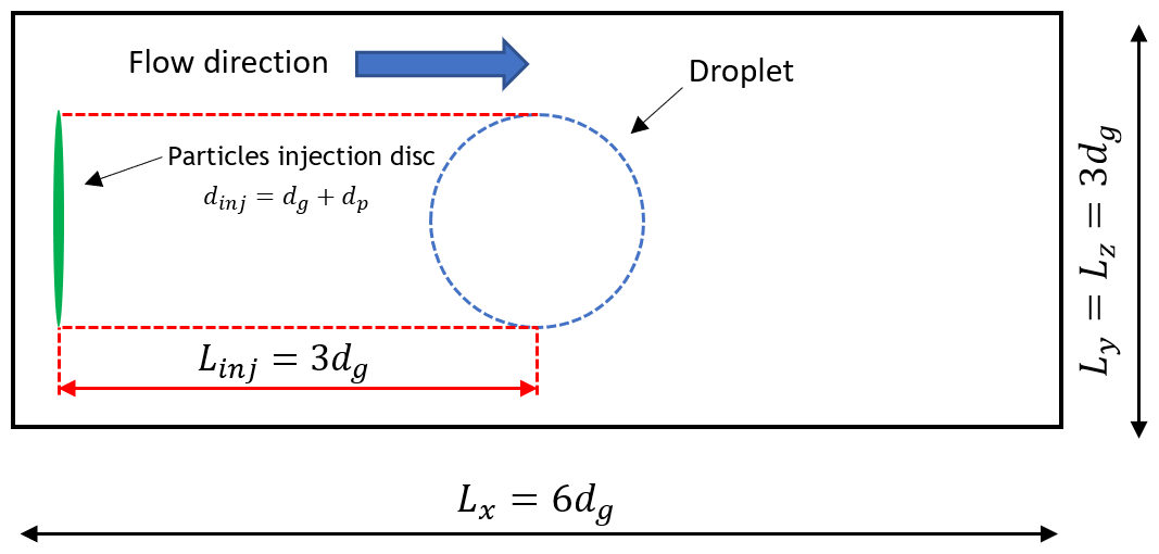
The simulation domain is set to be proportional to the size of the drop, i.e., 6 times d_d in length and 3d_d in depth and width (this results in the domain having the proportions of $\mathrm{2}:\mathrm{1}:\mathrm{1}$; see Fig. 3). Outflow boundary conditions are imposed for all faces of the domain except for the bottom, which can be a wall or an injection depending on the manner of initialization.

To keep the mesh cells cubic, we chose the number of points to be used in a 3D case to be $\mathrm{256}\times \mathrm{128}\times \mathrm{128}$ and, further, $\mathrm{512}\times \mathrm{256}\times \mathrm{256}$. As different sizes of drops are considered, the dimensionless parameter to be considered for comparing these simulations is $d_{\mathrm{g}}/\mathrm{\Delta }x$, which represents the number of mesh points inside the drop diameter, these being 42.7 and 85.3 mesh points for our two meshes.

The initialization condition corresponds to a drop falling in air at rest, starting from its theoretical terminal velocity, as shown in Fig. 2. This approach reduces the expensive simulation time required for the droplet to reach its terminal velocity from rest. In this case, the bottom boundary condition is set to wall type (Tanguy, 2004).

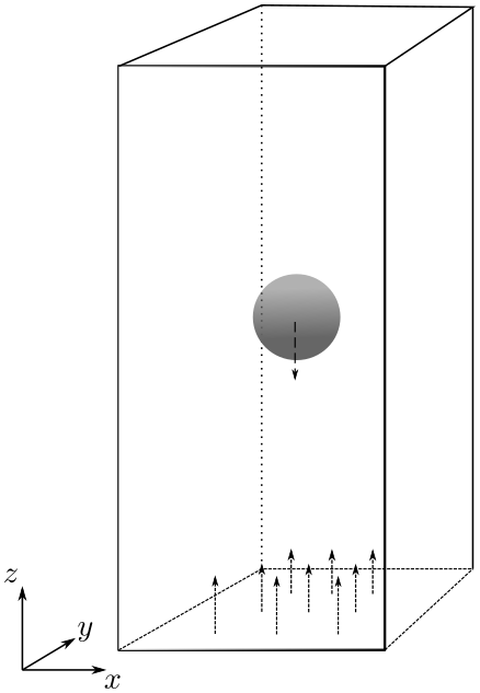
Figure 2 Initialization of the domain using either the configuration of the falling drop (arrow from the drop), with its theoretical terminal velocity present inside of the drop, or initialization of the theoretical terminal velocity at the bottom of the domain (arrows from the bottom).

Figure 3 Domain of the simulation.

An alternate initialization method of the flow was also tested for the highest Reynolds numbers. It corresponds to an initially motionless drop onto which the air is blown at theoretical terminal velocity from the bottom of the domain. This design aims to reduce the transient time required to eliminate the initial flow perturbations resulting from the nonphysical nature of the original initialization condition, where these perturbations might also be reflected in the drop's oscillations. The impact of using this different initialization condition is shown in Sect. 6 below. This alternate initialization is denoted as the blowing configuration in contrast to the falling drop configuration.

4.2 Steady-state criteria

The time advancement of the simulation continues until the drop reaches its terminal fall regime, for which the aerosol capture efficiency is sought. This terminal regime is considered to be reached when a set of parameters such as the terminal velocity, the mean axis ratio, and the oscillation frequency converge towards the literature reference values.

To qualify whether this state is achieved, we introduce the dimensionless time parameter t^⋆ as the ratio of the physical time t to the integral timescale of the flow past the drop T:

$$\begin{array}{}\text{(16)}& t^{\star }=t/T;\text{ with: }T={\displaystyle \frac{d_{\mathrm{d}}}{{\mathit{U}}_{\mathrm{\infty }}}},\end{array}$$

with U_∞ being the theoretical terminal velocity of the drop (Beard, 1976).

4.2.1 Axis ratio

The axis ratio (α) is defined as the ratio between the vertical (z direction) and horizontal (x or y) Feret diameters of the drop at each time, given by the following:

$$\begin{array}{}\text{(17)}& \mathit{\alpha }\left(t\right)={\displaystyle \frac{max\left(z\right|\mathit{\varphi }=\mathrm{0})-min(z|\mathit{\varphi }=\mathrm{0})}{max\left(x\right|\mathit{\varphi }=\mathrm{0})-min(x|\mathit{\varphi }=\mathrm{0})}},\end{array}$$

where $max\left(z\right|\mathit{\varphi }=\mathrm{0})$ corresponds to the maximum value of z for which an interface (given by ϕ=0) is detected.

The value found in the literature corresponds to the mean axis ratio over time.

4.2.2 Oscillation frequencies

The oscillation frequency is defined as the oscillation frequency of the axis ratio (Eq. 17). It is extracted from the fast Fourier transform (FFT) of the axis ratio time evolution in a steady-state regime.

4.2.3 Oscillation amplitudes

The oscillation amplitudes quantify the maximum extent of the deformations experienced by the drop. Their calculation is presented by the following equation:

$$\begin{array}{}\text{(18)}& A_{\mathit{\alpha }}=max\left(\mathit{\alpha }\right(t\left)\right)-min\left(\mathit{\alpha }\right(t\left)\right).\end{array}$$

4.3 Particle initialization

The particles are introduced into the computational domain following the procedure developed by Cherrier et al. (2016) and Dépée et al. (2021) (Fig. 3). In this approach, the particles are initialized within a virtual disk (shown in green in Fig. 3) located 3d_d upstream of the drop center. Their initial radial positions are randomly assigned within this disk of diameter $d_{\text{inj}}=d_{\mathrm{d}}+d_{\mathrm{p}}$ to ensure a homogeneous initial distribution. The initial particle velocity is set as the fluid velocity at the position of the injected particle (no slip velocity with respect to the fluid).

The particle diameters in the simulation vary within a range from 2 nm to 20 µm. A density of 1000 kg m⁻³ is used so that the geometric and aerodynamic diameters are equal.

4.4 Statistical convergence of trajectories

Since Brownian motion is a stochastic process, the convergence of the particle collection efficiency with respect to the number of particles tracked is evaluated by means of Student's t test (with a chosen 95 % confidence interval) (Student, 1908) after verifying the normality of the data with a Shapiro–Wilk test (Shapiro and Wilk, 1965). This procedure is inspired by Cherrier et al. (2016) and Dépée et al. (2021).

4.5 Particle flow time coupling

Up to Reynolds numbers of 260 (Re<260), water drops remain perfectly spherical (Beard et al., 1989), and the flow around them is known to be stationary (Pruppacher et al., 1998). These properties are not imposed by the methodology used here, which leaves the interface free, allowing the resolution for the non-stationary flow. Nevertheless, sphericity and stationarity are reproduced by the present model for Re<260 (see Sect. 5 and the Video Supplements, Reyes, 2025). In these cases, Lagrangian particle tracking is therefore performed on “frozen” flows obtained at steady state.

For Re>260, our simulations show oscillations of the drops, associated with unsteady flows when the terminal settling velocity is reached. Thus, fully coupled Lagrangian tracking is performed for these cases.

Additionally, a so-called snapshot method is tested as a possible means of reducing the computational time required to derive particle collection efficiencies. This method consists, first, of selecting instantaneous snapshots of the flow field, uniformly distributed in time over several periods of the oscillating steady-state regime. Second, particle Lagrangian tracking is performed for each of these frozen velocity fields, and the average particle behavior over all snapshots is derived. This method is expected to give identical results to the time-coupled approach, with a reduced computational effort, if the characteristic flow modulation time is long compared to the particle transit time in the domain.

5 Results for spherical-drop regimes

The approach is first verified and validated in the range of Reynolds numbers for which drops are perfectly spherical (Re<260), which is well documented in the literature. Here we adopt the definition of AIAA (1998) for the model verification and validation (V&V): validation is “the process of determining the degree to which a model is an accurate representation of the real world from the perspectives of the intended uses of the model”, and verification is “the process of determining that a model implementation accurately represents the developer’s conceptual description of the model and the solution to the model”.

For drops known to remain perfectly spherical at terminal velocity based on the literature (Re<260; Pruppacher et al., 1998; Beard and Chuang, 1987), the following parameters are verified:

• grid independence of the velocity field and drop terminal velocity;

• statistical convergence of particles collection efficiencies (see Sect. 4.4), evidenced through confidence intervals;

• independence of particle collection efficiencies with respect to the grid resolution used for the carrier phase and to the fluid velocity interpolation scheme (see Sect. 3.2).

Then, the model is validated by comparison with the following reference data:

• the drop terminal velocity, with the measurements by Beard (1976);

• the velocity field for the two continuous phases, with the simulation data of Cherrier et al. (2016);

• particle collection efficiencies, with the simulation data of Cherrier et al. (2016).

As stated in the Introduction, the simulation data of Cherrier et al. (2016) were chosen as the reference as they cover the widest range of Reynolds numbers and aerosol aerodynamic diameters. These data link the purely Brownian and purely inertial behaviors of the aerosol particles and retrieve data from other authors, whether analytical, numerical, or experimental (Cherrier et al., 2016; Dépée et al., 2021).

5.1 Verification and validation for the continuous phases

Figure 4 presents a qualitative comparison for a Re=30 simulated drop, as well as the streamlines of the flow. Figures 5 and 6 compare the velocity profiles computed for two grid resolutions and that reported by Cherrier et al. (2016) for Re=30 and 70, on two axes passing by the drop center: along the gravity direction (z axis) and on the y axis. Reference profiles of Cherrier et al. (2016) are plotted for comparison. It can be seen that the finest mesh reproduces the behavior of the velocity inside and outside the drop with good agreement. Nevertheless, half a radius away from the drop in the y direction, velocity profiles divert from reference data regardless of the mesh used. This suggests that the boundary conditions may be too close to the drop to accurately capture the flow at that distance. However, this should not affect the trajectories of particles close to the interface.

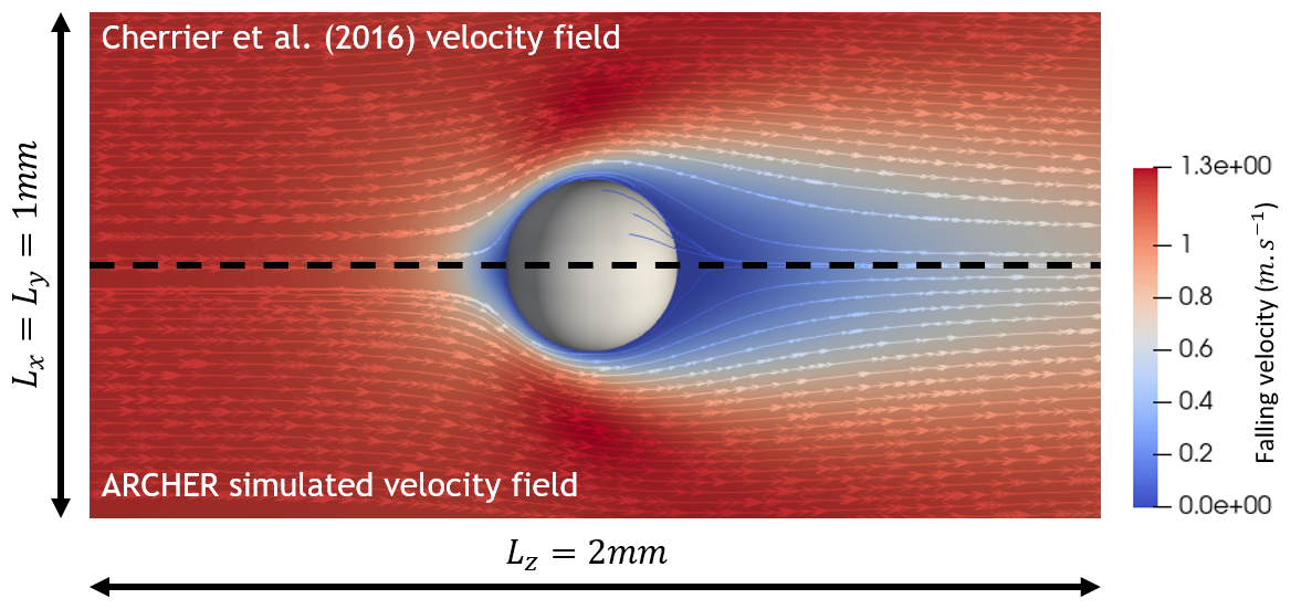
Figure 4 Stationary flow from Cherrier et al. (2016) for a drop of Re=30 compared to the one from the present simulation.

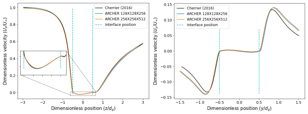
Figure 5 Velocity profiles comparisons for our Re=30 simulations and Cherrier et al. (2016) simulations.

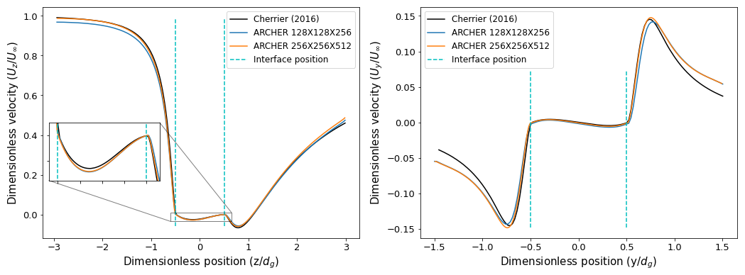
Figure 6 Velocity profiles comparisons for our Re=70 simulations and Cherrier et al. (2016) simulations.

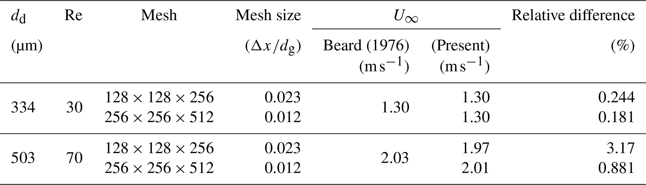
Additionally, Table 1 reports the computed terminal velocity and the corresponding reference values of Beard (1976). Results show that, regarding the predicted flow field and terminal velocity of the drop, grid-independent results are already obtained for a $\mathrm{128}\times \mathrm{128}\times \mathrm{256}$ grid, with differences of 0.24 % and 3.16 % in relation to the terminal velocity for Reynolds drops of 30 and 70, respectively. Refinement on a $\mathrm{256}\times \mathrm{256}\times \mathrm{512}$ grid leads to variations in velocities smaller than 0.90 %.

Beard (1976)

Table 1 Obtained terminal velocities for drops of Reynolds numbers 30 and 70 for two mesh sizes.

5.2 Verification and validation for the discrete phase

For the flow field being verified and validated for the carrier phase, the verification and validation process is pursued for aerosol particle dynamics. Figures 7 and 8 thus present the collection efficiency obtained for Re=30 and Re=70, respectively, for the two different mesh resolutions employed and for the two fluid velocity interpolation schemes employed. The corresponding reference data of Cherrier et al. (2016) are plotted for validation.

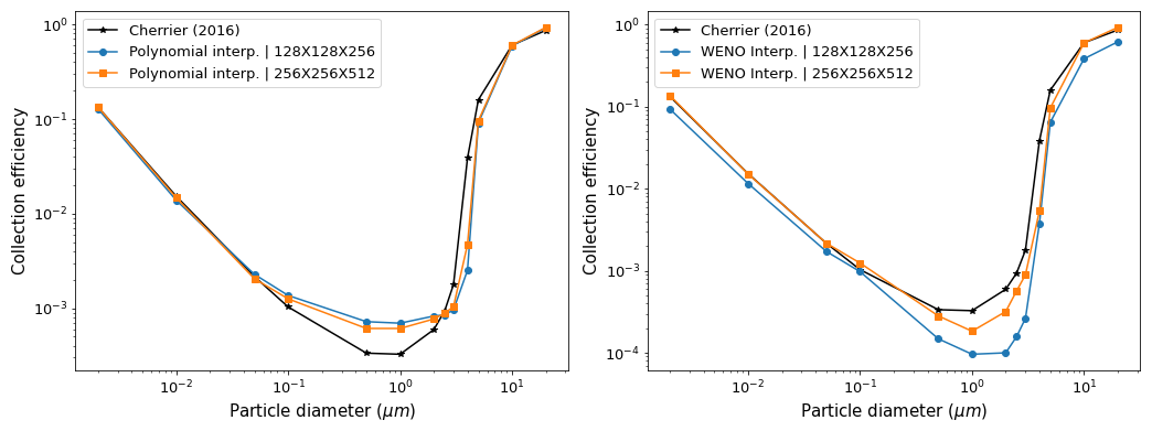
Figure 7 Collection efficiency results for an Re=30 drop using different configurations: polynomial interpolation (left) and WENO interpolation (right) and comparison with Cherrier et al. (2016) (black curve).

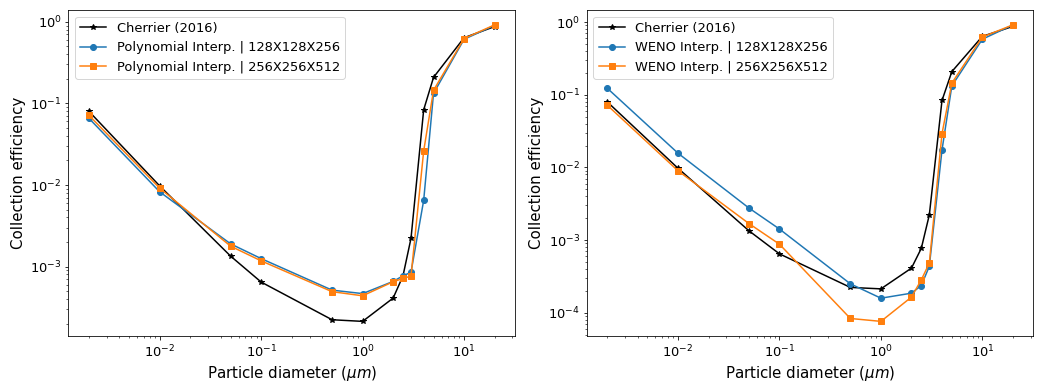
Figure 8 Collection efficiency results for an Re=70 drop using polynomial interpolation (left) and WENO interpolation (right) and comparison with Cherrier et al. (2016) (black curve).

The results show a grid convergence towards the reference results of Cherrier et al. (2016). However, a slight difference persists, even with the finest employed mesh, for particle in the Greenfield gap. The Greenfield gap (Greenfield, 1957) refers to the range of particle diameters for which the collection efficiency is at its minimum (ranging from approximately 50 nm to 3 µm here). We determined that this discrepancy is associated with velocity field interpolation inaccuracies at the particle position when the particle is close to the interface, where the interpolation schemes, within their stencil, take velocities that are part of the velocities inside the drop. This effect is particularly noticeable for Greenfield gap particles that show long grazing trajectories since they behave almost like perfect fluid tracers (Belut, 2019). For these trajectories, minor interpolation errors easily lead to erroneous capture of particles by the drop surface.

Overall, results exhibit the highest accuracy for particles with purely Brownian (d_p≲50 nm) or purely inertial (d_p≳3 µm) behavior. For these size ranges, the predicted collection efficiency differs from the reference by less than 6 % and 1 % for the polynomial and WENO interpolation schemes, respectively, with the finest mesh employed.

Hence, with regards to the collection efficiency, both interpolation methods converge to reference values as the flow mesh size decreases. However, Fig. 9 shows that a spatial bias of particle collection patterns on the drop surface exists for the polynomial interpolation scheme and not for the WENO scheme. This is exemplified in this figure by the initial and final positions of particles captured by the drop surface (for Re=70 and d_p=2 µm). Spurious alignment of the final particle positions is found for the polynomial scheme, while these final positions should be distributed following a statistically axially symmetric pattern.

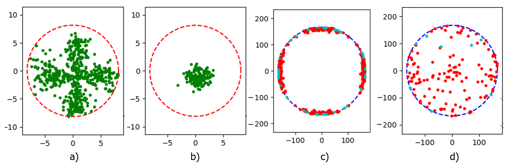
Figure 9 Initial (a, b) and final (c, d) positions of captured aerosol particles for d_p=2 µm and Re=70 using polynomial (a, c) and WENO (b, d) interpolation, respectively (coordinates in µm). For initial-position graphs (a, b), the dashed line marks the perimeter of the injection disk; for final-position graphs (c, d), the dashed line marks the drop cross-section, red dots correspond to particle impacts on the drop front face (streamwise), and light-blue dots correspond to particle impacts on the rear face.

Subsequently, only the WENO scheme is retained to interpolate the fluid velocity at the particles location since it appears to be both more precise and less spatially biased than the polynomial scheme. Regarding these results, the finest tested mesh ($\mathrm{256}\times \mathrm{256}\times \mathrm{512}$) provides the most accurate agreement with Cherrier et al. (2016), and, therefore, this will be the mesh used for further simulations.

In conclusion, the selected mesh resolution provides a robust resolution of continuous phase dynamics while maintaining the absolute error for aerosol collection efficiency in the Greenfield gap at a level of 10⁻³. In this regime, the primary collection mechanisms – Brownian motion and inertia – are minimal, rendering the calculation of E highly sensitive to numerical artifacts. Specifically, velocity inaccuracies at particle locations and interpolation-induced oscillations introduce significant errors. Although the implementation of a WENO scheme enhances accuracy and mitigates nonphysical particle alignment with the grid, the mesh density remains the limiting factor in achieving a precision better than 10⁻³. This drawback will remain for the non-spherical oscillating-drop regimes that are examined further on. It should be noted that Cherrier et al. (2016) had to use a spatial resolution that was 2.3 times higher in the vicinity of the drop interface to obtain grid-independent results on the collection efficiency in an axisymmetric 2D space and that such a resolution is beyond our current computational capabilities in DNS.

6 Results for non-spherical oscillating-drop regimes

We will now consider the case of deforming drops falling at Re>500. Computations are performed for drop diameters of 1.39 and 2 mm, corresponding to terminal Reynolds numbers of 500 and 876, respectively (see the online supplementary animations, Reyes, 2025). In this flow regime, the droplets experience noticeable deformations, oscillations, and vortex releases (see Table 2); also, much fewer reference data exist for validation.

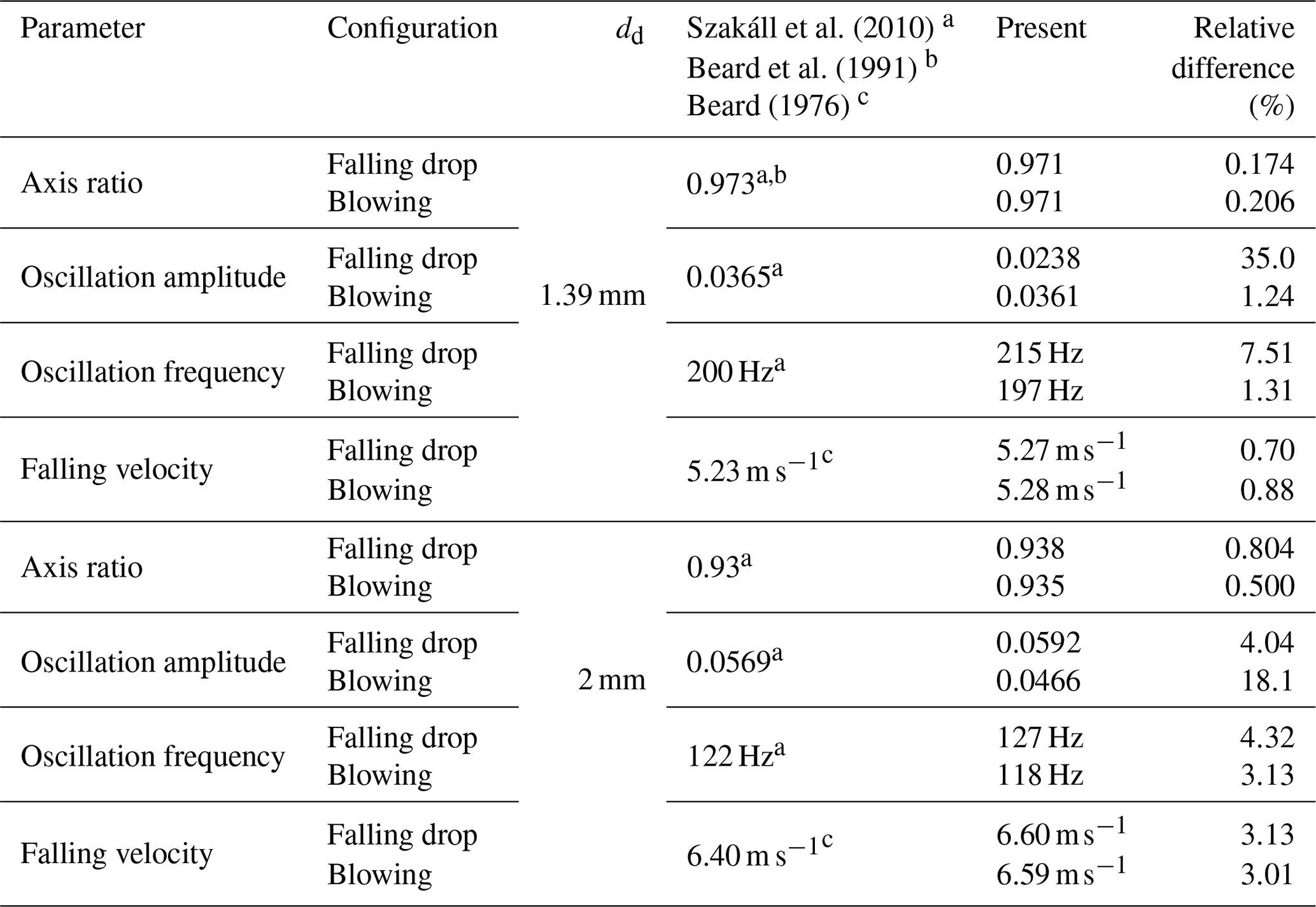
Szakáll et al. (2010)Beard et al. (1991)Beard (1976)

Table 2 Main dynamic data obtained for the continuous phases and comparison with results from Szakáll et al. (2010) and Beard (1976) for both initialization conditions.

6.1 Verification and validation for the continuous phases

For deformable drops, modeling verifications for the motion of the continuous phases are carried out with regard to the following:

• the independence of drop terminal velocity, mean axis ratio, and oscillation frequency from the initialization condition (falling drop vs. blowing configuration);

• the statistical stationarity of drop velocity and axis ratio.

The model is then validated by comparison with the following reference data:

• drop terminal velocity, with the measurements by Beard (1976);

• drop mean axis ratio and oscillation frequency, with the data of Szakáll et al. (2010).

6.1.1 Independence from initialization condition

The influence of the flow initialization method (i.e., the falling-drop configuration or the blowing configuration) is examined below, in Fig. 10, which shows the temporal evolution of the axis ratio and terminal velocity for both configurations for a 1.39 mm drop (Re=500). Experimental reference data by Beard (1976) and Beard et al. (1991) are also shown for comparison.

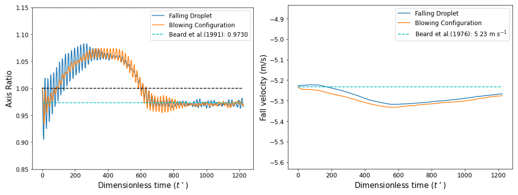
Figure 10 Evolution of axis ratio (left) and the falling velocity of the drop (right) over time for a 1.39 mm drop.

For both configurations, a similar temporal evolution of the axis ratio and terminal velocity is found. In the early stages of the simulation, the drop undergoes oscillations that result in an elongated, prolate shape (Fig. 11, left), characterized by an axis ratio exceeding unity, as the wake of the drop develops. For both initialization methods, there is a period of fast fluctuations visible in Fig. 10 (left). They represent shape perturbations due to the imposed initial velocity in the first initialization method (blue line), as expected above in the context of Fig. 2. Meanwhile, the second initialization method (orange line) allows for the dumping of these primary perturbations (for t<400). Here, however, once the droplet picks up the momentum from the surrounding airflow ($\mathrm{400}<t<\mathrm{800}$), secondary oscillations appear, only to dissipate once fall velocity is reached. In both cases, this oscillatory behavior is transient, and a stationary oscillatory regime with an oblate drop shape (Fig. 11, right) is reached while the axis ratio converges towards the values reported in the literature (Beard et al., 1991). During the early transient stage, the drop's fall velocity increases slightly and then tends asymptotically towards the value of the Beard (1976) model, coinciding with the moment when the axis ratio also enters its relaxation stage.

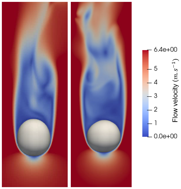
Figure 11 Different flow velocities and morphologies for a 2 mm drop, with a prolate shape (left) (at 250 t^⋆) corresponding to the initial transient phase which later acquires an oblate shape (right) (at 605 t^⋆).

No significant influence of the chosen initialization condition is observed on the mean axis ratio, oscillation frequency, and terminal velocity in the pseudo-stationary regime. The physical (and computational) time necessary to reach steady state is also identical for both initialization strategies. Steady state is reached after 677 and 448 t^⋆ for the 1.39 and 2 mm drop diameters, respectively. Hence, further on, we retain only the use of the blowing configuration as the initialization.

6.1.2 Physical parameters at drop-settling velocity

Drop terminal velocity, mean axis ratio, oscillation amplitude, and oscillation frequency are extracted from the pseudo-stationary regime reached by the drop and are presented in Table 2 together with literature reference data for the two considered drop diameters (1.39 and 2 mm). For these four quantities, the deviations from available experimental data are, respectively, less than 3 %, 0.5 %, 18 %, and 3 % for the Reynolds tested and the simulations' blowing configurations. The coupled flow dynamics in and around the drop appear to be correctly captured by the model. Ultimately, compared to the state of the art in simulating the dynamics of a water droplet in free fall (Balla et al., 2019), our model successfully reproduces the spontaneous destabilization of an initially spherical water droplet into the oscillatory dynamics observed experimentally (Szakáll et al., 2010; Szakall et al., 2009).

6.2 Verification and validation for the discrete phase

Having assessed the quality of the modeling of the continuous phases, we now turn to the evaluation of the modeling of the discrete phase. We examine first the effect of the chosen time-coupling method (fully time-coupled Lagrangian tracking vs. snapshot method; see Sect. 4.5).

6.2.1 Effect of time-coupling method on E

In this section, the necessity of a fully unsteady simulation is evaluated for a 2 mm drop in free fall (Re=876). We first present results obtained with the snapshot method: collection efficiencies E are determined using a series of Lagrangian particle trackings performed on frozen flow fields during different phases of the drop oscillation. Figure 12 (left) shows the efficiencies obtained for the ϕ_i time positions shown in the inset. For readability, statistical uncertainties of E arising from repeated Lagrangian tracking (see Sect. 4.4) are not shown here. We observe that, for similar phases in the oscillation cycle (similar α and $\dot{\mathit{\alpha }}$), comparable collection efficiencies are calculated (e.g.,: $E_{{\mathit{\varphi }}_{\mathrm{2}}}\approx E_{{\mathit{\varphi }}_{\mathrm{6}}}$). In contrast, the collection efficiencies obtained for drop shapes that are similar but in phase opposition during the oscillation cycle (similar α but opposite $\dot{\mathit{\alpha }}$) exhibit significant differences, especially around the minimum of efficiency (e.g.,: $E_{{\mathit{\varphi }}_{\mathrm{2}}}\ne E_{{\mathit{\varphi }}_{\mathrm{4}}}$, especially for d_p≈2 µm). This result suggests that the collection efficiency is influenced not only by the shape of the drop, which logically dictates geometric contact, but also by its deformation dynamics, which induce significant changes in the flow within the gas boundary layer and, consequently, in the collection efficiency.

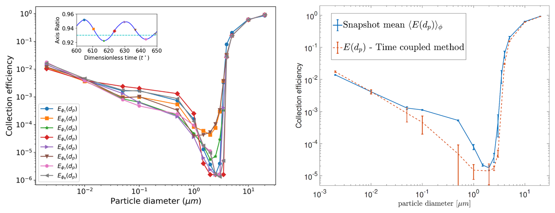
Figure 12 Collection efficiencies calculated for different snapshots of the drop oscillation cycle (left) and the comparison between their corresponding mean 〈E(d_p)〉_ϕ and time-coupled simulation (right).

The mean numerical efficiency 〈E(d_p)〉_ϕ over the entire oscillation cycle of the drop is then shown in Fig. 12 (right). It is calculated as the average of E(d_p) over computed snapshots ϕ_i, i.e., $\langle E\left(d_{\mathrm{p}}\right){\rangle }_{\mathit{\varphi }}={\sum }_{i=\mathrm{1}\mathrm{\dots }\mathrm{8}}{E}_{{\mathit{\varphi }}_i}\left(d_{\mathrm{p}}\right)$. The uncertainty of 〈E(d_p)〉_ϕ arising from the limited number of snapshots used and from the number of Lagrangian trackings used for each snapshot is computed by classical error propagation, assuming both effects are uncorrelated. The largest relative statistical uncertainties on 〈E(d_p)〉_ϕ are found for dp=3 µm.

The collection efficiency obtained with Lagrangian tracking coupled in time with the flow is also shown in Fig. 12 (right) for comparison. For this result, Lagrangian tracking is performed during the full simulated stationary oscillating regime, i.e., between $t^{\star }=\mathrm{605}$ and $t^{\star }=\mathrm{1000}$.

It is apparent from Fig. 12 (right) that the snapshot method and the time-coupled method provide similar results outside the Greenfield gap, i.e., for inertia-dominated particles (d_p≳3 µm) and diffusion-dominated particles (d_p≲50 nm), while collection efficiencies predicted by the two methods differ by up to 1 order of magnitude in the intermediate region, where no particular collection mechanism dominates. This behavior is easily explained by recognizing the tracer behavior of Greenfield gap particles, which are therefore the most sensitive to flow modulations, taken wrongly into account by the snapshot method. This underscores the necessity of performing Lagrangian tracking coupled in time with the flow to accurately capture the collection efficiency in the Greenfield gap.

We may add that the snapshot method is based on the assumption that the flow seen by the particles is quasi-stationary. This is justifiable if the characteristic times of drop oscillation and flow modulation are large compared with the transit time of the particles around the drop. In practice, drop oscillation periods are, respectively, 19 and 27 t^⋆ for Reynolds numbers of 500 and 876: hence, these periods are actually comparable to the mean particle transit times around the drop (which typically range between 10 and 20 t^⋆ for the particle diameters considered, as shown in Belut, 2019). This explains why the snapshot method is not reliable here.

6.2.2 Comparison with experimental measurement of E

For deforming and oscillating drops falling at terminal velocity, few validation experimental data exist regarding their aerosol collection efficiencies (Lai et al., 1978; Quérel et al., 2014). When these data are available, the knowledge of the true size distribution of employed aerosol particles is of particular importance since the collection efficiencies vary very sharply with particle size (as visible in Figs. 7, 8, and 12). To the best of our knowledge, the measurements from Quérel et al. (2014) are the only ones found in the literature with an accurate aerosol size distribution: we thus employ those for validation. However, Quérel et al. (2014) measured mass collection efficiencies over a whole particle size distribution and not number collection efficiencies resolved with particle sizes. Hence, presently, simulated collection efficiencies first need to be converted into equivalent collection efficiencies before performing the comparison. The experimentally equivalent mass collection efficiency E_m is computed by integrating E(d_p) over the experimental probability density function (PDF) of aerosol particles diameters following

$$\begin{array}{}\text{(19)}& E_{\mathrm{m}}\left(f\right)={\displaystyle \frac{{\int }_{\mathrm{0}}^{\mathrm{\infty }}E\left(d_{\mathrm{p}}\right)f\left(d_{\mathrm{p}}\right)d_{\mathrm{p}}^{\mathrm{3}}\mathrm{d}{d}_{\mathrm{p}}}{{\int }_{\mathrm{0}}^{\mathrm{\infty }}f\left(d_{\mathrm{p}}\right)d_{\mathrm{p}}^{\mathrm{3}}\mathrm{d}{d}_{\mathrm{p}}}},\end{array}$$

where f(dp) is the experimentally measured number probability density function of aerosol particle diameters, provided by Quérel et al. (2014). E_m is hence defined for each experimentally tested aerosol probability density function f. With these PDF values being characterized through their mass mean particle diameter d_m with $d_{\mathrm{m}}=\frac{{\int }_{\mathrm{0}}^{\mathrm{\infty }}{d}_{\mathrm{p}}f\left(d_{\mathrm{p}}\right)d_{\mathrm{p}}^{\mathrm{3}}\mathrm{d}{d}_{\mathrm{p}}}{{\int }_{\mathrm{0}}^{\mathrm{\infty }}f\left(d_{\mathrm{p}}\right)d_{\mathrm{p}}^{\mathrm{3}}\mathrm{d}{d}_{\mathrm{p}}}$, we adopt the same abscissa d_m as Quérel et al. (2014) and compare E_m(d_m) obtained either numerically in the present work or experimentally by Quérel et al. (2014) in Fig. 13.

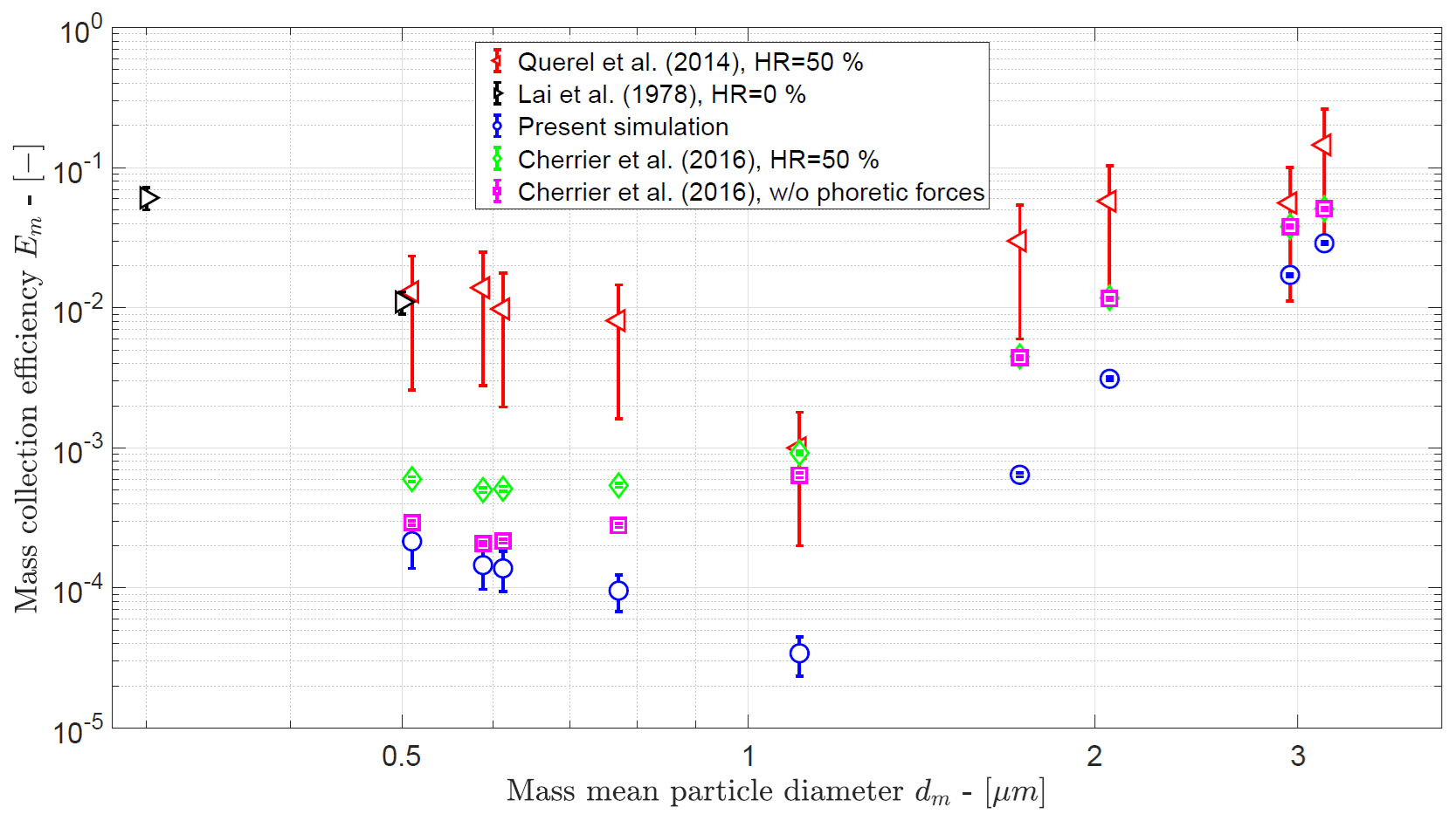
Figure 13 Mass collection efficiencies obtained under the experimental conditions of Quérel et al. (2014) for a 2 mm drop in free fall (Re=876): measurements versus simulations and existing correlations.

Note that the experimental results of Quérel et al. (2014) were obtained under sub-saturated air conditions (relative humidity close to 50 %), indicating the existence of diffusiophoretic (Ebel et al., 1988) and thermophoretic (Talbot, 1981) forces acting on aerosols due to drop evaporation, while current numerical results do not take these forces into account. For reference, Fig. 13 also displays the following:

• collection efficiencies measured by Lai et al. (1978), for which the exact aerosol particle PDF is unknown and for which the carrier gas is nitrogen (presumably 0 % humidity and active phoretic forces);

• theoretical values obtained by integrating the correlation for E proposed by Cherrier et al. (2016) for experimental PDF f (as in Eq. 19) under the operating conditions of Quérel et al. (2014) (RH=50 %). This correlation extends the correlation of Wang et al. (1978) with particle inertia effect and thus takes into account phoretic forces, particle inertia, and Brownian diffusion;

• theoretical values obtained similarly with the correlation of Cherrier et al. (2016) but without the contribution of phoretic forces.

Note that the correlation of Wang et al. (1978) extended by Cherrier et al. (2016) is used here beyond the drop Reynolds range for which it was established (Re⪅200 with no drop deformation and/or oscillation). This model therefore provides approximate results, which only allow for an appreciation of the order of magnitude of the impact of phoretic forces, as a possible cause of the discrepancy between simulation results and experimental measurements. In Fig. 13, uncertainties are derived by classical error propagation from Eq. (19), taking into account statistical uncertainties of E(d_p) and experimental uncertainties of f(d_p). The uncertainties of the results of Cherrier et al. (2016) account solely for experimental uncertainties of f(d_p) provided by Quérel et al. (2014).

Figure 13 shows that measurements from Quérel et al. (2014) and Lai et al. (1978) are similar. However, as Lai et al. (1978) provide neither the size distribution of the aerosol particles nor the relative humidity, it is preferable to compare our model to Quérel et al. (2014). We see that both theoretical and experimental collection efficiencies present the usual “V” shape trend, with a minimum of efficiency for d_m≈1 µm (Greenfield gap). However, all models underestimate measurements by, typically, 1 order of magnitude, and the uncertainties considered are not sufficient to explain the differences. Assuming that the model of Wang et al. (1978), extended by Cherrier et al. (2016), provides a fair approximation of the magnitude of phoretic effects under the conditions of the experiment, it seems that phoretic forces are also not sufficient to explain the discrepancies (the predicted increase in E does not exceed a 2-fold increase). However, we cannot rule out the limitations of these models, which are based on the assumption of a spherical symmetry of vapor and temperature fields around the drop, with a first-order correction to account for non-negligible Reynolds numbers that break this symmetry. This approximation is not calibrated for the present situation that involves drop Reynolds numbers higher than 200: Lemaitre et al. (2020) recently hypothesized, based on a comparison between their experimental results and the Wang et al. (1978) model (and, subsequently, Cherrier et al., 2016's model), that the correlation underestimates phoretic effects for larger drops. To evaluate this hypothesis, the methodology could be extended to determine more exactly the contribution of phoretic forces in this drop size range by resolving energy and vapor mass fraction conservation equations around the evaporating drop, but this is beyond the scope of the present article.

In summary, for a 2 mm drop experiencing deformation and oscillation, the model fails to retrieve the available E measurements within 1 order of magnitude. The two main reasons are, on the one hand, the steepness of the collection efficiency rise in the inertial regime, which makes E very sensitive to small uncertainties in particle diameters, and, on the other hand, the diminishing of E in the Greenfield gap, which makes the signal-to-noise ratio very small in this particle size range: the result is a high sensitivity to measurement uncertainties or numerical errors. Beyond these general remarks, it is difficult to attribute the discrepancy between simulations and experiments to one particular cause as several factors clearly contribute to it. The first is, of course, the numerical uncertainty in particle trajectories already mentioned, linked to the imprecision of air velocity calculated at particle position. Future work will have to focus on improving this accuracy. A second factor of uncertainty arises from the hygrometry and temperature conditions under which the validation data of Quérel et al. (2014) were obtained: under these conditions of low relative humidity (RH=50 %) and thermal imbalance, the drops present a non-negligible evaporation rate, with a gradient of vapor fraction and temperature at the liquid–gas interface. These gradient induces diffusion-phoresis and thermophoresis on the particles, which are known to increase collection efficiency in the Greenfield gap by, typically, 1 order of magnitude (Wang et al., 1978; Cherrier et al., 2016). These effects are not taken into account in the present simulations, which correspond to the isothermal case without evaporation. In the present case, the bias induced by not taking these phoretic forces into account can be roughly evaluated using correlations for E from the literature, as shown in Fig. 13. These correlations suggest that phoretic forces could explain an increase in E by a factor of 2, which is still far from the discrepancy existing between simulations and experiments, which is more in the ratio of 20:1. This evaluation is approximate, however, as the correlations of Cherrier et al. (2016) and Wang et al. (1978) are not established for Re⪆200. Finally, the last factor likely to contribute significantly to the discrepancy between simulations and experiments is metrological for, as already mentioned, E measurement remains a delicate exercise sensitive to numerous difficulties, in particular the control of electrostatic charges on drops and aerosols, which can greatly increase collection efficiency (Wang et al., 1978; Dépée et al., 2021), and the control of test aerosol particle sizes. Indeed, Quérel et al. (2014)'s measurements are based on the mass of collected particles, and a very small number of particles of larger diameter than those measured could have affected the measurements since such particles are not only very efficiently collected but also contribute to the total mass in proportion to the cube of their diameter. The existence of such particles in the experiment cannot be ruled out due to aggregation phenomena (linked to the high aerosol concentrations required to obtain a measurable efficiency) and due to the inherently partial control of aerosol size distribution in the experiment (sampling-based control). It should also be noted that the aerosol particles used were hygroscopic and that an increase in their diameter during the experiment, due to heterogeneous nucleation of water vapor cannot be ruled out. In addition, the flow upstream of the drops in the experiments may not have been at rest as in the simulations. Upstream turbulence could potentially affect the collection efficiency. All of these possible experimental biases make it difficult to isolate the role of any particular mechanism.

7 Conclusion

A DNS–VOF–level set approach was coupled to Lagrangian discrete particle tracking to model the scavenging of airborne particles by a single free-falling water drop, making it possible to take into account the effect of the complex drop dynamics on particle scavenging in the cases of oscillating regimes and drop deformation. The effects of both drag force and Brownian motion on particle trajectories were accounted for.

This approach enables us to predict the main physical quantities associated with fluid flows inside and outside the drop, as well as the dynamics of the gas–liquid interface: for the stationary laminar regime (Re=30 and 70), the drop's terminal velocity, the sphericity of its interface, and the internal and external velocity profiles are all correctly predicted. For the unsteady regime with interface deformation and oscillation, the results are validated in terms of drop terminal velocity, mean axis ratio, and axis ratio oscillation amplitude and frequency. For these four quantities, the deviations from available experimental data are, respectively, less than 3 %, 0.5 %, 18 %, and 3 % for the tested Reynolds numbers of 500 and 876 and for the blowing configuration of simulations.

For the dispersed-aerosol phase, validation by comparison with literature data is less conclusive. In the fall regime where drops remain spherical, the collection efficiency E is both qualitatively and quantitatively accurate: a maximum deviation of 10⁻³ for E is observed in the Greenfield gap, where E is at its minimum, using the finest tested mesh and the WENO interpolation scheme. Compared to the physical range of variation of E, the inaccuracy of the present model remains small for spherical drops. On the other hand, under unsteady conditions with deformation and oscillation of the drop, only an indirect validation is proposed by comparison with Quérel et al. (2014), where measurements of E are integrated over poly-disperse particle size distributions. The found deviations between simulations and experiments for E typically reach 1 order of magnitude in the aerosol size range tested, even though the typical (V-shaped) trend of collection efficiency as a function of aerosol size is correctly predicted. Such a difference is significant but in line with the variability found in the literature for this parameter and with both numerical and experimental uncertainties.

The paper also evaluated the interest of deriving E from Lagrangian trackings performed on flow snapshots over the drop oscillation cycle. This method was found to be suitable for particles outside the Greenfield gap (presently for d_p≲50 nm or d_p≳3 µm) but not inside the Greenfield gap. Flow–particle time coupling is then recommended.

In conclusion, this article reports on a first attempt to simulate the collection of aerosols by a deformable water drop falling transiently through still air. While the flow dynamics of the continuous phases appear to be correctly predicted, the results highlight a number of points for improvement in the prediction of the dynamics of the dispersed phase: the accuracy of interpolation of air velocity at the particle position in the drop boundary layer; the need for coupled dynamic calculation for all three phases; and the interest, for certain ambient conditions, of taking into account heat exchange and water phase changes to account for the contributions of phoretic forces and Stefan flow to capture. To validate modeling, further experimental work is also required to eliminate uncertainties relating to the control of aerosol diameters, upstream turbulence, and phoretic forces. The collection of aerosol particles by deformable free-falling drops is therefore still a matter of research.

Appendix A

A1 Lagrange polynomial interpolation

To interpolate any scalar Φ (i.e., level set, velocity component) in 3D on a point $(x,y,z)$ with an N-degree polynomial $P(x,y,z)$, we have the following formula:

$$\begin{array}{}\text{(A1)}& \begin{array}{rl}& P(x,y,z)=\sum _{k=\mathrm{0}}^N\sum _{j=\mathrm{0}}^N\sum _{i=\mathrm{0}}^N{\mathrm{\Phi }}_{i,j,k}{L}_i^{\left(x\right)}\left(x\right)L_j^{\left(y\right)}\left(y\right)L_k^{\left(z\right)}\left(z\right),\\ & \text{with}\\ & L_i^{\left(x\right)}\left(x\right)=\prod _{l=\mathrm{0},l\ne i}^N{\displaystyle \frac{x-x_l}{x_i-x_l}},\\ & L_j^{\left(y\right)}\left(y\right)=\prod _{m=\mathrm{0},m\ne j}^N{\displaystyle \frac{y-y_m}{y_j-y_m}},\\ & L_k^{\left(z\right)}\left(z\right)=\prod _{n=\mathrm{0},n\ne k}^N{\displaystyle \frac{z-z_n}{z_k-z_n}}.\end{array}\end{array}$$

In the case of N=2, used here for level set and velocities, the 27-point stencil is centered on the particle, and no specific treatment is done for velocity near the interface. That means gas and liquid velocities can be used together to approximate these on the particle and to assess any errors in interpolation evaluation due to discontinuities of velocity gradients.

A2 WENO interpolation

The weighted essentially non-oscillatory (WENO) schemes represent a class of high-order accurate schemes specifically engineered for solving problems characterized by piecewise smooth solutions that may contain discontinuities. The fundamental concept behind these schemes revolves around the precision of the approximation process. Instead of employing a fixed stencil for interpolation, WENO schemes utilize a nonlinear adaptive approach.

This adaptive procedure dynamically selects the locally smoothest stencils, effectively minimizing the risk of crossing or interpolating through discontinuities within the domain. Without this selection, the interpolation process might inadvertently incorporate, in the same stencil, velocity information from both sides of the interface, potentially leading to erroneous interpolated values, especially where velocity gradient jumps occur at the interface, as in the present case.

Then, because we are within a finite volume framework, any velocity component $\stackrel{\mathrm{‾}}{u}$ of U given by the Navier–Stokes solver is a cell-averaged function. The fifth WENO (or ENO) approaches initially developed by Shu (1997) permit us to interpolate velocity at the center of a particle or to compute an average velocity inside a volume containing the particle. Both are developed and converge when r_p≪Δx, but only the second method is detailed here.

A two-dimensional schematic of this procedure is found in Fig. A1. The desired average velocity (noted as U_f and standing for any component of the velocity) is inside the dashed square ($S_{\mathrm{p}}=[x_{\mathrm{p}}-r_{\mathrm{p}},x_{\mathrm{p}}+r_{\mathrm{p}}]\times [y_{\mathrm{p}}-r_{\mathrm{p}},y_{\mathrm{p}}+r_{\mathrm{p}}]$) surrounding the particle p, whose center of mass is located in the control volume ${\mathrm{\Omega }}_{i,j}^{\stackrel{\mathrm{‾}}{u}}=[x_{i-\mathrm{1}/\mathrm{2}},x_{i+\mathrm{1}/\mathrm{2}}]\times [y_{j-\mathrm{1}/\mathrm{2}},y_{j+\mathrm{1}/\mathrm{2}}]$ of the corresponding velocity component $\stackrel{\mathrm{‾}}{u}$.

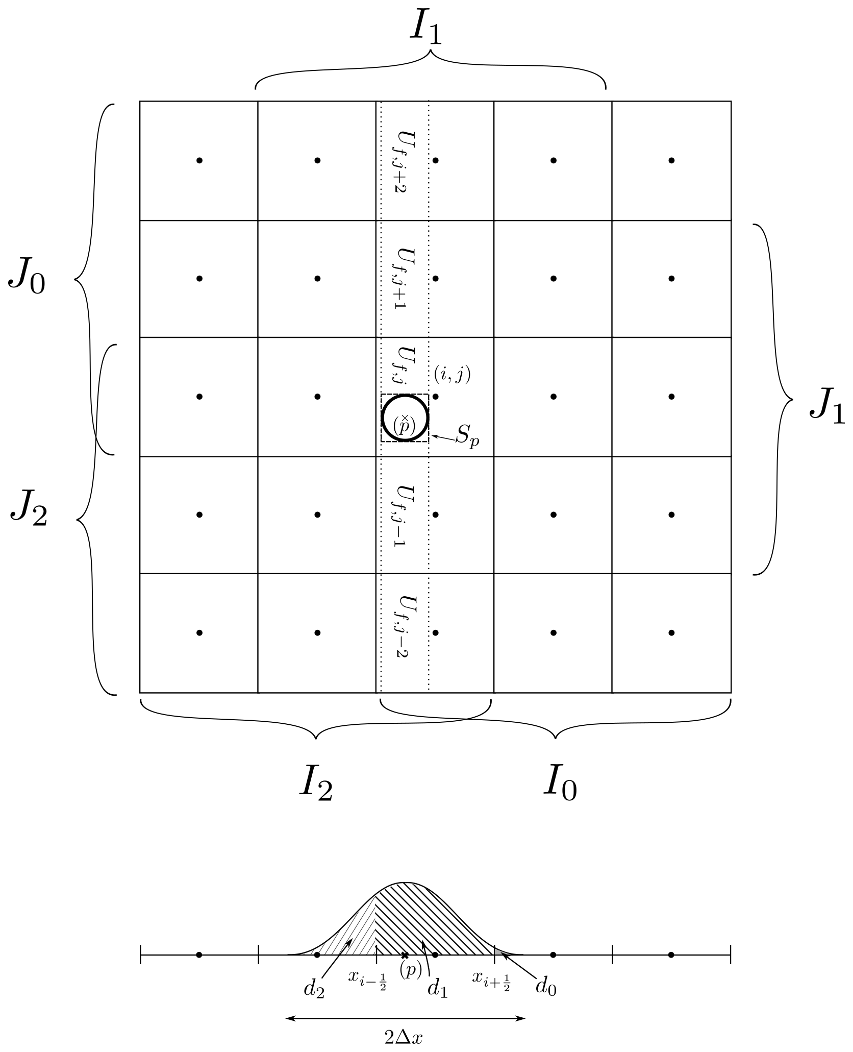
Figure A1 Illustration of 2D, 25-point stencil used to interpolate the mean velocity on a square surrounding the particle. I_r and J_r represent the sub-stencil in the x direction and y direction, respectively. The coefficient d_r used to weight the velocity computed by each stencil (I_r here) is symbolized by the area under a sinusoidal curve of a period equalling 2Δx and centered on the particle position.

The mean velocities $U_{f,j-\mathrm{2}}\mathrm{\dots }{U}_{f,j+\mathrm{2}}$ are first computed with the help of interpolation in the x direction, and then the average velocity U_f on S_p is determined by interpolation of these values in the y direction.

The computation of U_f,j follows

$$\begin{array}{}\text{(A2)}& U_{f,j}=\sum _{r=\mathrm{0}}^{k-\mathrm{1}}{\mathit{\omega }}_r\left(x_{\mathrm{p}}\right)U_{f,j}^{\left(r\right)}\left(x_{\mathrm{p}}\right),\end{array}$$

where k=3 for the fifth WENO. In Eq. (A2), $U_{f,j}^{\left(r\right)}\left(x_{\mathrm{p}}\right)$ is computed with the help of velocity values inside the stencil I_r,

$$U_{f,j}^{\left(r\right)}\left(x_{\mathrm{p}}\right)=\left(F_j^{\left(r\right)}\right(x_{\mathrm{p}}+r_{\mathrm{p}})-F_j^{\left(r\right)}(x_{\mathrm{p}}-r_{\mathrm{p}}\left)\right){\displaystyle \frac{\mathrm{\Delta }x}{\mathrm{2}\times r_{\mathrm{p}}}},$$

and the following approximation of a primitive of velocity (Shu, 1997):

$$\begin{array}{}\text{(A3)}& \begin{array}{rl}{F}_j^{\left(r\right)}& \left(x\right)-K\\ & =\sum _{s=\mathrm{0}}^{k-\mathrm{1}}{\stackrel{\mathrm{‾}}{u}}_{i-r+s,j}\sum _{m=s+\mathrm{1}}^k\prod _{\underset{l\ne m}{l=\mathrm{0}}}^k{\displaystyle \frac{x-x_{i-r+l-\frac{\mathrm{1}}{\mathrm{2}}}}{x_{i-r+m-\frac{\mathrm{1}}{\mathrm{2}}}-x_{i-r+l-\frac{\mathrm{1}}{\mathrm{2}}}}}\\ & =\sum _{s=\mathrm{0}}^{k-\mathrm{1}}{c}_{rs}\left(x\right){\stackrel{\mathrm{‾}}{u}}_{i-r+s,j}.\end{array}\end{array}$$

The weighted coefficients ω_r(x_p) in Eq. (A2) are defined by the following:

$$\begin{array}{}\text{(A4)}& {\mathit{\omega }}_r\left(x_{\mathrm{p}}\right)={\displaystyle \frac{{\mathit{\alpha }}_r\left(x_{\mathrm{p}}\right)}{{\sum }_{k=\mathrm{0}}^{k-\mathrm{1}}{\mathit{\alpha }}_k\left(x_{\mathrm{p}}\right)}},\end{array}$$

with the “MwenoZ” method (Hu et al., 2016) being used to compute α_r(x_p) (also β_r, ϵ, and ζ) coefficients.

$$\begin{array}{}\text{(A5)}& {\mathit{\alpha }}_r\left(x_{\mathrm{p}}\right)=d_r\left(x_{\mathrm{p}}\right)(\mathrm{1}+{\displaystyle \frac{\mathit{\zeta }}{{\mathit{\beta }}_r+\mathit{ϵ}}})\end{array}$$

Generally, d_r(x_p) coefficients are computed in such a way, allowing the recovery of the fifth order in a smoothed region. Because particles are mobile – i.e the coefficients d_r have to be recalculated at each time step – the stability condition ω_r>0 ∀r is, in general, not respected (Shu, 1997; Shi et al., 2002). This might imply the appearance of non-physical particle trajectories. Thus, we have decided to weight each stencil using a sinusoidal function (Eq. A6) whose argument is relative to the particle position x_p, as presented at the bottom of Fig. A1, ensuring that it takes only positive values. A consequence of this, however, is the loss of the fifth order in the smoothed region.

$$\begin{array}{}\text{(A6)}& \begin{array}{rl}{d}_{\mathrm{0}}& ={\displaystyle \frac{\mathit{\pi }}{\mathrm{4}\mathrm{\Delta }x}}\underset{x_{i+\mathrm{1}/\mathrm{2}}}{\overset{x_{\mathrm{p}}+\mathrm{\Delta }x}{\int }}\cos \left({\displaystyle \frac{\mathit{\pi }}{\mathrm{2}\mathrm{\Delta }x}}\right(x-x_{\mathrm{p}}\left)\right)\mathrm{d}x\\ d_{\mathrm{1}}& ={\displaystyle \frac{\mathit{\pi }}{\mathrm{4}\mathrm{\Delta }x}}\underset{x_{i-\mathrm{1}/\mathrm{2}}}{\overset{x_{i+\mathrm{1}/\mathrm{2}}}{\int }}\cos \left({\displaystyle \frac{\mathit{\pi }}{\mathrm{2}\mathrm{\Delta }x}}\right(x-x_{\mathrm{p}}\left)\right)\mathrm{d}x\\ d_{\mathrm{2}}& ={\displaystyle \frac{\mathit{\pi }}{\mathrm{4}\mathrm{\Delta }x}}\underset{x_{\mathrm{p}}-\mathrm{\Delta }x}{\overset{x_{i-\mathrm{1}/\mathrm{2}}}{\int }}\cos \left({\displaystyle \frac{\mathit{\pi }}{\mathrm{2}\mathrm{\Delta }x}}\right(x-x_{\mathrm{p}}\left)\right)\mathrm{d}x\end{array}\end{array}$$

Finally, the same procedure is applied in the y direction, where the velocity on the particle is as follows:

$$U_f=\sum _{r=\mathrm{0}}^{k-\mathrm{1}}{\mathit{\omega }}_r\left(y_{\mathrm{p}}\right)U_f^{\left(r\right)}\left(y_{\mathrm{p}}\right),$$

with

$$U_f^{\left(r\right)}=\left(G^{\left(r\right)}\right(y_{\mathrm{p}}+r_{\mathrm{p}})-G^{\left(r\right)}(y_{\mathrm{p}}-r_{\mathrm{p}}\left)\right){\displaystyle \frac{\mathrm{\Delta }y}{\mathrm{2}\times r_{\mathrm{p}}}}$$

and

$$\begin{array}{}\text{(A7)}& \begin{array}{rl}& G^{\left(r\right)}\left(y\right)-K\\ & =\sum _{s=\mathrm{0}}^{k-\mathrm{1}}{U}_{f,j-r+s}\sum _{m=s+\mathrm{1}}^k\prod _{\underset{l\ne m}{l=\mathrm{0}}}^k{\displaystyle \frac{y-y_{j-r+l-\frac{\mathrm{1}}{\mathrm{2}}}}{y_{j-r+m-\frac{\mathrm{1}}{\mathrm{2}}}-y_{j-r+l-\frac{\mathrm{1}}{\mathrm{2}}}}}\\ & =\sum _{s=\mathrm{0}}^{k-\mathrm{1}}{c}_{rs}\left(y\right)U_{f,j-r+s}.\end{array}\end{array}$$

The global method therefore uses a 125-point stencil in three dimensions, and, because velocity components have different locations, this procedure differs for each of them.