Simulation of aerosol transport, evaporation and scattering in the Evaporative Light Scattering Detector – Part 2

This study presents a comprehensive model for simulating aerosol dynamics and signal response in the Evaporative Light Scattering Detector (ELSD), a widely used analytical technique in liquid and supercritical fluid chromatography. The model integrates a zero-dimensional model including droplet atomization, convection, impingement, evaporation and finally light scattering of the droplet cloud. The physically based model includes chemical species properties, operational settings and environmental conditions. The model accounts for complex phenomena such as multi-component evaporation, particle impingement and size-dependent light scattering. The use of computational fluid dynamic (CFD) simulations provides detailed insights into flow characteristics within the ELSD geometry and allows estimation of the droplet losses by impingement. Model predictions are compared against experimental data for various analytes and solvents across a range of concentrations and temperatures. The model accurately captures experimentally measured trends for volatile and semi-volatile species, but discrepancies are observed for non-volatile analytes at higher temperatures. The present simulations are the very first framework for modelling ELSD operation, and the developed model provides the first tool for optimizing detector performance and interpreting results in chromatographic applications.

1 Introduction

The Evaporative Light Scattering Detector (ELSD) is an analytical technique used in combination with liquid and supercritical fluid chromatography for the detection of separated analytes, with extensive applications in the pharmaceutical, biomaterial and food manufacturing industries (Mourey and Oppenheimer, 1984). Functionally similar to analyte detection methods such as UV–Vis spectroscopy, the ELSD distinguishes itself by detecting solutes via light scattering. This characteristic enables it to be marketed as a universal detector due to its ability to detect analytes that do not absorb in the IR and UV–Vis region. The operational principle of the ELSD involves several steps. The solution containing analytes separated by chromatographic techniques is atomized. The atomized solution passes through a heated tube, where the solvent is evaporated, leaving behind dry analyte particles. These particles are subsequently detected in the form of light scattered by a laser beam, allowing the ELSD to detect analytes that are less volatile than the mobile phase (Lafosse et al., 1992). The process underscores the versatility and broad applicability of the ELSD in various analytical contexts.

Although the ELSD is a well-established analytical technique for the detection of analytes, the physics behind its operation are is well characterized. Quantitative models detailing aerosol behaviour which are sensitive to analyte volatility and varying volumetric flow rates are absent from the literature. This work introduces a zero-dimensional model which takes in the chemical species involved (analyte, liquid solvent and drying gas) and ELSD operational settings (gas and liquid flow rates, analyte concentration, and evaporator tube temperature) as inputs to simulate the resultant ELSD signal response. This is achieved via construction of a system-wide transfer function which links outputs to inputs of sequential model components. The model connects simulations of liquid injector breakup, flow, aerosol transport and evaporation, diluent and analyte thermodynamic properties, and scattering models, with minimal input from experimental constants where necessary. A companion study describes the experimental methods and results which are used for comparison with the model outputs (Bertani et al., 2026). Further details of the models and experimental results used for comparisons are available in the PhD thesis by Bertani (2024).

2 Model description

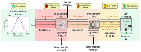
The geometry and dimensions for the inner tubing of the ELSD are outlined in Figs. 1 and 2. The model solves steady-state conservation equations that describe the motion and evaporation of an initial particle size distribution along the flow system containing an initial concentration of analyte. Steady analyte concentration was used for validation experiments, even though the analyte concentration may be variable with time, in which case it is assumed that the operation is quasi-steady with respect to analyte concentration. A schematic of the model is shown in Fig. 2 as a diagram and in Fig. 1 as a series of subroutines. The geometric and flow parameters for the system are outlined in Table 1.

Figure 1 Cross-section of ELSD geometry. Each numbered section is simulated in a separate module.

Figure 2 Outline of different sections of the model with relevant equations for each stage.

Table 1 ELSD sections indicating relevant dimensions and bulk velocities.

The bulk flow velocity in each section, unless otherwise stated, is determined from the total gas flow rate and local section area, u_g = $Q_{\mathrm{g}}/A$.

Module 1 corresponds to the determination of the inlet condition. The particle concentration and corresponding diameter distribution is based on an atomization model which takes as inputs the geometry of the nebulizer, the gas and liquid flow rates, and fluid properties. The model used to determine the particle size distribution at the inlet condition in Module 1 is discussed in more detail in Sect. 3.1.

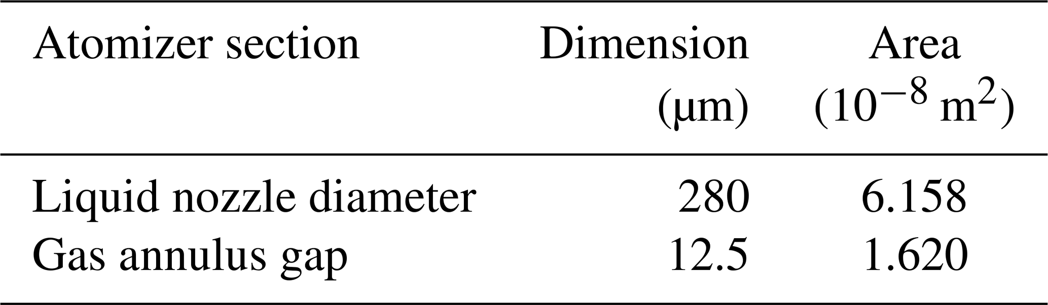
The spray is produced using a twin-fluid coaxial SeaSpray high-performance nebulizer (Glass Expansion), whose geometry is summarized in Fig. 3 and Table 2.

Figure 3 (a) SeaSpray high-performance nebulizer and (b) cross-sectional diagram depicting the nozzle tip showing liquid nozzle and gas annulus.

Table 2 Dimensions associated with the ELSD nebulizer.

Models described in Modules 2 and 3 in Fig. 1 collect the particle size and velocity distribution from Module 1, solve the equation of motion for particles of a given size class across the length of the module, and determine what fraction of those particles is transmitted across the two barriers along the pathway as follows:

• a.

  Y junction. The high-speed spray meets the Y junction (Module 2 in Fig. 1), where large droplets impact the wall and are collected as waste, while smaller droplets follow the flow and continue towards the optical chamber.

• b.

  Diffuser cartridge. The flow is diverted at the diffuser cartridge (Module 3 in Fig. 1) which consists of a series of rings and counter-rings which act as impaction plates (see Appendix D for a detailed cross-section). Again, large droplets precipitate out and are no longer used in the calculation, and the overall ratio of the liquid to droplet mass flow rate is decreased.

Module 4 in Fig. 1 consists of the evaporation tube. The model solves the equation of motion for the droplets of different sizes, as well as the corresponding droplet evaporation during the residence time. The evaporation model is discussed in more detail in Sect. 3.4.

Module 5 finally translates the resulting droplet number distribution as a function of droplet diameter to simulate the detection of remaining particles in the optical chamber. The model is discussed in detail in Sect. 3.5. The optical chamber is outfitted with a continuous 480 nm laser beam crossing the flow of aerosol, with a photo-detector fixed at an angle of 60 ° to the laser source for detection of the scattered light by the particles.

3 Model components

3.1 Atomization

The first section of the model generates the initial droplet distribution used for the simulation for a custom set of operational conditions. Part of this section overlaps with the description in the companion paper by Bertani et al. (2026). Measurements of air-blast-generated droplet distributions suggest that droplets emerge according to a log-normal diameter distribution:

$$\begin{array}{}\text{(1)}& p\left(d_{\mathrm{p}}\right)={\displaystyle \frac{\mathrm{1}}{d_{\mathrm{p}}\mathit{\sigma }\sqrt{\mathrm{2}\mathit{\pi }}}}\exp \left(-{\displaystyle \frac{{\left(\ln d_{\mathrm{p}}-\mathit{\mu }\right)}^{\mathrm{2}}}{\mathrm{2}{\mathit{\sigma }}^{\mathrm{2}}}}\right),\end{array}$$

where p(d_p) is the normalized probability distribution function of droplets of size d_p. Log-normal distributions are controlled by the parameters μ and σ, which are the distribution mode and width, respectively, in logarithmic space. A related metric is the Sauter mean diameter (SMD), D₃₂, which represents the mean ratio of volume to area of the droplets. Given an assumed log-normal distribution, the SMD is related to the log-normal parameter μ via Hinds and Zhu (2022):

$$\begin{array}{}\text{(2)}& D_{\mathrm{32}}=\exp \left(\mathit{\mu }+{\displaystyle \frac{\mathrm{3}}{\mathrm{2}}}{\mathit{\sigma }}^{\mathrm{2}}\right).\end{array}$$

Investigations in the companion paper by Bertani et al. (2026) lay out the procedure for experimental measurements of the incoming spray particle size distribution and the final results on particle number distribution downstream of the nebulizer. The study obtained measurements of the mean incoming droplet size distribution using a combination of phase Doppler particle analysis (PDPA) and aerosol aerodynamic classification (AAC). Scaling of the measurements for solvent fluids with different properties relies on previous measurements of the Sauter mean diameter (SMD) D₃₂ for similar air blast nebulizers by Aliseda et al. (2008). Log-normal distributions measured by Aliseda et al. (2008) for twin-fluid concentric pneumatic nebulizers similar to the current one were used as a validated baseline for a range of compounds whose physical properties are well within the range of industrially relevant solvents. The particular values of μ and σ for the validation case were determined experimentally in the companion study (Bertani et al., 2026). The same authors offered an equation linking the D₃₂ of the initial droplet distribution to the solvent properties as follows:

$$\begin{array}{}\text{(3)}& \begin{array}{rl}{\displaystyle \frac{D_{\mathrm{32}}}{D_{\mathrm{L}}}}=& C_{\mathrm{1}}\left(\mathrm{1}+m_r\right){\left({\displaystyle \frac{b_{\mathrm{g}}}{D_{\mathrm{L}}}}\right)}^{\mathrm{1}/\mathrm{2}}{\left({\displaystyle \frac{{\mathit{\rho }}_{\mathrm{L}}}{{\mathit{\rho }}_{\mathrm{g}}{\mathit{Re}}_{b_{\mathrm{g}}}}}\right)}^{\mathrm{1}/\mathrm{4}}{\displaystyle \frac{\mathrm{1}}{\sqrt{{\text{We}}_{D_{\mathrm{L}}}}}}\\ & \cdot \left(\mathrm{1}+C_{\mathrm{2}}{\left({\displaystyle \frac{D_{\mathrm{L}}}{b_{\mathrm{g}}}}\right)}^{\mathrm{1}/\mathrm{6}}{\left({\displaystyle \frac{{\mathit{Re}}_{b_{\mathrm{g}}}}{{\mathit{\rho }}_L/{\mathit{\rho }}_{\mathrm{g}}}}\right)}^{\mathrm{1}/\mathrm{12}}{\text{We}}_{D_{\mathrm{L}}}^{\mathrm{1}/\mathrm{6}}{\text{Oh}}_{D_{\mathrm{L}}}^{\mathrm{2}/\mathrm{3}}\right),\end{array}\end{array}$$

where D_L is the liquid orifice diameter; m_r is the ratio of liquid to gas flow; b_g is taken as the thickness of the atomizer gas annulus (Aliseda et al., 2008); and ρ_L and ρ_g are densities of the liquid and gas, respectively. The non-dimensional numbers ${\mathit{Re}}_{b_{\mathrm{g}}}$ are based on the atomizer gas annulus and properties, We${}_{D_{\mathrm{L}}}$ is the Weber number based on the liquid properties and nozzle diameter, and ${\text{Oh}}_{D_{\mathrm{L}}}$ is the Ohnesorge number based on liquid properties and jet diameter. The constants C₁ and C₂ were experimentally determined in the same study to be 1.734 and 1.0, respectively.

Once D₃₂ is obtained for the particular fluid via Eq. (3), the inlet probability distribution function (pdf) is obtained via Eq. (1). The final droplet number concentration N is obtained via conservation of liquid mass flow rate for the droplets:

$$\begin{array}{}\text{(4)}& Q_{\mathrm{L}}=Q_{\mathrm{g}}N\underset{\mathrm{0}}{\overset{\mathrm{\infty }}{\int }}p\left(d_{\mathrm{p}}\right){\displaystyle \frac{\mathit{\pi }}{\mathrm{6}}}{d}_{\mathrm{p}}^{\mathrm{3}}\mathrm{d}\left(d_{\mathrm{p}}\right).\end{array}$$

The initial velocity of the droplets at the outlet of the atomizer is assumed to be the same as that of the surrounding gas, which is the local speed of sound in the choked flow, with a velocity of u_g = 318 m s⁻¹ at the relevant nebulizer operating conditions. Particles start slowing down immediately due to drag owing to the surrounding gas. The value for u_g in the atomization chamber was obtained from CFD simulations (see Sect. 6.1) across the whole ELSD from atomizer tip to optical detector and was taken to be represented by the value of the velocity at the centreline of the cross-section.

3.2 Equation of motion

The equation of motion for a spherical particle of diameter d_p moving along the duct with a velocity of u_p = $\frac{\mathrm{d}{x}_{\mathrm{p}}}{\mathrm{d}t}$ and surrounded by gas at a velocity u_g is given as follows:

$$\begin{array}{}\text{(5)}& {\displaystyle \frac{\mathrm{d}{x}_{\mathrm{p}}}{\mathrm{d}t}}=u_{\mathrm{p}}\text{(6)}& {\displaystyle \frac{\mathrm{d}{u}_{\mathrm{p}}}{\mathrm{d}t}}={\displaystyle \frac{\mathrm{3}}{\mathrm{4}}}{\displaystyle \frac{C_{\mathrm{d}}}{d}}{\displaystyle \frac{{\mathit{\rho }}_{\mathrm{g}}}{{\mathit{\rho }}_{\mathrm{p}}}}\left(u_{\mathrm{g}}-u_{\mathrm{p}}\right)\left|u_{\mathrm{g}}-u_{\mathrm{p}}\right|,\end{array}$$

where the drag coefficient C_d = $\frac{F_{\mathrm{d}}}{\frac{\mathrm{1}}{\mathrm{2}}{\mathit{\rho }}_{\mathrm{g}}{\left|u_{\mathrm{p}}-u_{\mathrm{g}}\right|}^{\mathrm{2}}}=\frac{C_{\mathrm{d}}^{*}}{C_{\mathrm{c}}}$ is extracted from theory and experiments as (Hinds and Zhu, 2022)

$$\begin{array}{}\text{(7)}& C_{\mathrm{d}}^{*}=\left\{\begin{array}{ll}\frac{\mathrm{24}}{\mathit{Re}},& \text{for}\mathit{Re}\le \mathrm{1}\\ \frac{\mathrm{24}}{\mathit{Re}}\left(\mathrm{1}+\frac{{\mathit{Re}}^{\mathrm{2}/\mathrm{3}}}{\mathrm{6}}\right),& \text{for}\mathrm{1}\ge \mathit{Re}\ge \mathrm{1000}\\ \mathrm{0.424},& \text{for}\mathit{Re}\ge \mathrm{1000}.\end{array}\right.\end{array}$$

Here the Reynolds number is based on the diameter of the particle, d_p, and the relative velocity between particle and gas, |u_p−u_g|. The relative velocity of the gas varies along the different sections, from very high at the inlet where droplets emerge to zero near the final evaporator section when small particles move at the same velocity as the gas.

The coefficient C_c is unity for particles much larger than the mean free path of the gas in the flow, λ, which is typically of the order of tens of nanometres. The correction is based on the Knudsen number, Kn = $\mathrm{2}\mathit{\lambda }/d$,

$$\begin{array}{}\text{(8)}& \mathit{Kn}={\displaystyle \frac{\mathrm{2}\mathit{\lambda }}{d}},\end{array}$$

and is given as

$$\begin{array}{}\text{(9)}& C_{\mathrm{c}}\left(\mathit{Kn}\right)=\mathrm{1}+\mathit{Kn}\left(\mathrm{1.257}+\mathrm{0.4}\exp \left(-{\displaystyle \frac{\mathrm{1.1}}{\mathit{Kn}}}\right)\right).\end{array}$$

The mean free path can be calculated as

$$\begin{array}{}\text{(10)}& \mathit{\lambda }={\displaystyle \frac{k_{B}T}{\sqrt{\mathrm{2}}p\mathit{\xi }}},\end{array}$$

where k_B is the Boltzmann constant, T is the gas temperature, p is the pressure, and ξ is the effective cross-sectional area of the gas particle. For nitrogen at 1 bar, λ = 34.5 nm.

3.3 Wall impingement

There are two sections where droplets of sufficient inertia may hit the walls and cease to be transported with the flow, namely the ELSD Y piece or diffuser cartridge. The transmission efficiency of the particles across an obstacle is expressed as a function of the ability of the flow to provide sufficient drag relative to particle inertia to allow the particle to follow the flow as it travels across the regions where the flow is forced through a corner. This is expressed as the Stokes number, Stk, which is the ratio of the characteristic particle stopping time to that of the flow time (Hinds and Zhu, 2022). A solution of Eq. (6) for Re < 1 yields a characteristic stopping time τ_s = $C_C\frac{{\mathit{\rho }}_{\mathrm{p}}{d}_{\mathrm{p}}^{\mathrm{2}}}{\mathrm{18}{\mathit{\mu }}_{\mathrm{g}}}$, leading to a Stokes number equal to

$$\begin{array}{}\text{(11)}& \mathit{Stk}=C_C{\displaystyle \frac{{\mathit{\rho }}_{\mathrm{p}}{d}^{\mathrm{2}}}{\mathrm{18}{\mathit{\mu }}_{\mathrm{g}}}}{\displaystyle \frac{u_{\mathrm{g}}}{L}},\end{array}$$

where τ_g = $L/u_{\mathrm{g}}$ is the characteristic flow time. Particles with motion characterized by Stk lower than unity follow the flow streamlines around obstructions, whereas they otherwise deviate from the gas flow streamlines and may impact obstacles. For particles with a Reynolds number larger than unity, there is no analytical solution to the stopping time, but the approximate correlations below based on Stokes number are still routinely used, with appropriate validation.

A collection efficiency C_eff(Stk) is defined as the fraction of total particle concentration of a given diameter (and thus Stokes number) in a flow lost to impaction onto an obstacle. For each impaction element, the ratio of the transmitted particle number concentration fraction to the incoming fraction is thus given as follows:

$$\begin{array}{}\text{(12)}& {\displaystyle \frac{N_{\mathrm{out}}}{N_{\mathrm{in}}}}=\mathrm{1}-C_{\mathrm{eff}}\left(\mathit{Stk}\right).\end{array}$$

The collection efficiency is often represented using the following expression (Hinds and Zhu, 2022):

$$\begin{array}{}\text{(13)}& C_{\mathrm{eff}}\left(\mathit{Stk}\right)={\displaystyle \frac{\mathrm{1}}{\mathrm{2}}}\left(\text{erf}\left(W\left(\sqrt{\mathit{Stk}}-\sqrt{{\mathit{Stk}}_{\mathrm{50}}}\right)\right)+\mathrm{1}\right),\end{array}$$

where erf is the error function, W is a non-dimensional parameter characterizing the width of the function in Stokes number space, and Stk₅₀ is the Stk value which gives a collection efficiency of 50 %. The values of these two parameters depend on the type of obstacle and are discussed further on. An example of the change in the particle concentrations and efficiency as a function of droplet diameter is shown in Fig. 4.

Figure 4 Example of a simulated droplet size distribution before and after the impingement loss for an obstacle. The value of d₅₀ is shown for the original distribution as a dashed line. The collection efficiency curve is also plotted against particle diameter.

In this study, collection efficiency curves were determined through a detailed investigation via CFD simulations of droplets in flows (see Sect. 6.2) and were fitted according to Eq. (13). Simulations were carried out for scenarios involving the Y piece and the diffuser cartridge, both of which act as impaction surfaces within the ELSD.

3.4 Evaporation model

The output from Module 2 described in the previous section is used as the input distribution for the evaporator tube section of the ELSD in Module 3. The model solves the equations for evaporation for a given diameter bin of a given size. The calculations assume that the original number concentration of particles remains constant during the evaporation process as the corresponding droplet diameter decreases over the convective time. Number concentrations can change by collision (which is neglected for the presently dilute mixture) or impaction (which is active only across the obstructions described in the previous section) and are considered to be negligible in the evaporation tube.

The following assumptions are made: (a) the temperature along the duct is constant. This is justified as the mixture is dilute, the tube walls operate with a feedback loop for constant temperature, and evaporation does not consume sufficient energy to change the temperature of the bath gas significantly. (b) The rate of evaporation is sufficiently low so that the vapour pressure of the evaporating droplet does not change the vapour pressure of the bulk mixture. The latter is assumed to correspond to its upper bound throughout the domain, corresponding to the molar fraction attained if all droplets did vapourize completely. Since the mixture is very dilute, this means there is very little change in bulk vapour pressure. (c) The vapour pressure at the surface of the evaporating material is assumed to be associated with the temperature of the droplet, which is assumed to remain constant during the process.

3.4.1 Rate of evaporation

The rate of evaporation is obtained by considering the evaporation rate of each class of droplet of a given initial diameter. In order to model the evaporation of solvents and high-vapour-pressure analytes, the Abramzon and Sirignano droplet evaporation model (Abramzon and Sirignano, 1989; Sirignano, 2010) was employed. The model describes the mass and energy transfer rates of uniform temperature and composition droplets by the following set of non-linear coupled differential equations:

$$\begin{array}{}\text{(14)}& {\displaystyle \frac{\mathrm{d}{m}_{\mathrm{m}}}{\mathrm{d}t}}=-\mathit{\pi }{d}_{\mathrm{p}}{\mathit{Sh}}^{*}{\stackrel{\mathrm{‾}}{\mathcal{D}}}_{\mathrm{v}}{\stackrel{\mathrm{‾}}{\mathit{\rho }}}_{\mathrm{g}}\ln \left(\mathrm{1}+B_{\mathrm{m}}\right)=\dot{m},\text{(15)}& {\displaystyle \frac{\mathrm{d}{m}_{\mathrm{T}}}{\mathrm{d}t}}=-\mathit{\pi }{d}_{\mathrm{p}}{\mathit{Nu}}^{*}{\displaystyle \frac{{\stackrel{\mathrm{‾}}{\mathit{\lambda }}}_{\mathrm{g}}}{{\stackrel{\mathrm{‾}}{c}}_{\mathrm{p},\mathrm{v}}}}\ln \left(\mathrm{1}+B_{\mathrm{T}}\right)=\dot{m},\text{(16)}& {\displaystyle \frac{\mathrm{d}{T}_{\mathrm{d}}}{\mathrm{d}t}}={\displaystyle \frac{\dot{m}}{m}}{\displaystyle \frac{\mathrm{1}}{c_{\mathrm{p},\mathrm{l}}}}\left(L_{\mathrm{v}}-{\displaystyle \frac{{\stackrel{\mathrm{‾}}{c}}_{\mathrm{p},\mathrm{v}}\left(T_{\mathrm{g}}-T_{\mathrm{d}}\right)}{B_{\mathrm{T}}}}\right).\end{array}$$

In the equations above, m_m = m_T = m is the mass of the droplet and enforces the fact that the rate of mass evaporation, $\dot{m}$, limited by the diffusivity of either mass or energy, must be the same and is solved for as an eigenvalue of the problem. In the equations above, d_p is the droplet diameter; Sh^* and Nu^* are the Sherwood and Nusselt numbers, both modified for non-zero convection rates; ${\stackrel{\mathrm{‾}}{\mathcal{D}}}_{\mathrm{v}}$ is the average binary diffusion coefficient between the evaporant and surrounding gas; ${\stackrel{\mathrm{‾}}{\mathit{\rho }}}_{\mathrm{g}}$ is the average gas density; ${\stackrel{\mathrm{‾}}{\mathit{\rho }}}_{\mathrm{l}}$ is the liquid density; B_m and B_T are the Spalding mass and energy transfer coefficients, respectively, defined further on; T_d is the instantaneous temperature of the droplet; T_g is the temperature of the gas in the far field; ${\stackrel{\mathrm{‾}}{\mathit{\lambda }}}_{\mathrm{g}}$ is the average thermal conductivity of the gas; ${\stackrel{\mathrm{‾}}{c}}_{\mathrm{p},\mathrm{v}}$ is the average specific heat capacity (at constant pressure) of the vapour in the gas mixture; c_p,l is the specific heat capacity of the liquid; ${\stackrel{\mathrm{‾}}{c}}_{\mathrm{p},\mathrm{g}}$ is the averaged specific heat capacity (at constant pressure) of the gas; and L_v is the latent heat of vaporization of the liquid.

Averaged properties, $\stackrel{\mathrm{‾}}{\mathit{\zeta }}$, use the film temperature according to the following:

$$\begin{array}{}\text{(17)}& \stackrel{\mathrm{‾}}{\mathit{\zeta }}={\mathit{\zeta }}_{\mathrm{s}}+{\displaystyle \frac{\mathrm{1}}{\mathrm{3}}}\left({\mathit{\zeta }}_{\mathrm{g}}-{\mathit{\zeta }}_{\mathrm{s}}\right),\end{array}$$

where the subscripts s and g represent surface or bulk gas flow.

The liquid is considered to be a binary mixture of solvent and analyte/solute. In order to take into account the evaporation of either, an extension of the original model is used, as validated by Brenn et al. (2007), in which the evaporation of either is considered to be independent:

$$\begin{array}{}\text{(18)}& {\displaystyle \frac{\mathrm{d}{m}_{\mathrm{tot}}}{\mathrm{d}t}}={\displaystyle \frac{\mathrm{d}{m}_{\mathrm{w}}}{\mathrm{d}t}}+{\displaystyle \frac{\mathrm{d}{m}_{\mathrm{sol}}}{\mathrm{d}t}},\end{array}$$

where $\frac{\mathrm{d}{m}_{\mathrm{tot}}}{\mathrm{d}t}$ represents the total rate of mass transfer from the droplet, and the individual rates of mass transfer are expressed independently by Eq. (14). In the case of analyte vaporization, droplet properties that may refer to liquid or solvent properties in Eq. (14) are replaced with properties relating to those of the solute. Equation (18) is solved until the total droplet mass is lower than or equal to the mass of the solute, (m_d ≤ m_sol), at which point the system solves for the further evaporation of the analyte only.

The equations for evaporation (Eqs. 14–16) are solved together with the equations of motion (Eqs. 5 and 6) until the displacement of the particles has reached the length of the evaporation tube. At this location, the diameter of the original size class is tallied as the final diameter. The new diameter distribution can then be accordingly determined since, by assumption, the number concentration for each original class, N(d), remains constant through the evaporation process.

3.4.2 Heat transfer correlations

The baseline Sherwood and Nusselt numbers are the normalized mass and heat transfer coefficients for a non-evaporating sphere according to Froessling (1938):

$$\begin{array}{}\text{(19)}& {\displaystyle }{\mathit{Sh}}_{\mathrm{0}}={\displaystyle \frac{h_{\mathrm{m}}{d}_{\mathrm{p}}}{\mathcal{D}}}=\mathrm{2}+\mathrm{0.552}{\mathit{Re}}^{\mathrm{1}/\mathrm{2}}{\mathit{Sc}}^{\mathrm{1}/\mathrm{3}},\text{(20)}& {\displaystyle }{\mathit{Nu}}_{\mathrm{0}}={\displaystyle \frac{h{d}_{\mathrm{p}}}{\mathit{\lambda }}}=\mathrm{2}+\mathrm{0.552}{\mathit{Re}}^{\mathrm{1}/\mathrm{2}}{\mathit{Pr}}^{\mathrm{1}/\mathrm{3}},\end{array}$$

where h_m and h are the convective mass and heat transfer coefficients, and d_p is the droplet diameter.

A correction is applied to the base correlation to account for the heat and mass loss via evaporation according to

$$\begin{array}{}\text{(21)}& \begin{array}{l}{\mathit{Sh}}^{*}=\mathrm{2}+\frac{{\mathit{Sh}}_{\mathrm{0}}-\mathrm{2}}{F\left(B_{\mathrm{m}}\right)},\\ {\mathit{Nu}}^{*}=\mathrm{2}+{\displaystyle \frac{{\mathit{Nu}}_{\mathrm{0}}-\mathrm{2}}{F\left(B_{\mathrm{T}}\right)}},\end{array}\end{array}$$

and F(B) is the correction factor for the film thickness due to Stefan flow and is defined as

$$\begin{array}{}\text{(22)}& F\left(B\right)=(\mathrm{1}+B{)}^{\mathrm{0.7}}{\displaystyle \frac{\ln (\mathrm{1}+B)}{B}},\end{array}$$

where B stands for the corresponding heat and mass transfer numbers.

The Spalding mass transfer number B_m is defined as follows:

$$\begin{array}{}\text{(23)}& B_{\mathrm{m}}={\displaystyle \frac{Y_{\mathrm{v},\mathrm{s}}-Y_{\mathrm{v},\mathrm{g}}}{\mathrm{1}-Y_{\mathrm{v},\mathrm{s}}}},\end{array}$$

where Y_v,s and Y_v,g are the mass fraction of vapour at the surface and in the bulk gas phase. The mass and molar fractions at the surface (subscript s) and in the far field (subscript g) are calculated as follows:

$$\begin{array}{}\text{(24)}& \begin{array}{l}{Y}_{\mathrm{v},\mathrm{s}}=\frac{X_{\mathrm{v},\mathrm{s}}{M}_{\mathrm{v}}}{X_{\mathrm{v},\mathrm{s}}{M}_{\mathrm{v}}+\left(\mathrm{1}-X_{\mathrm{v},\mathrm{s}}\right)M_{\mathrm{g}}},\\ X_{\mathrm{v},\mathrm{s}}={\displaystyle \frac{p_{\mathrm{v}}^{\mathrm{sat}}}{p_{\mathrm{g}}}},\\ Y_{\mathrm{v},\mathrm{g}}={\displaystyle \frac{X_{\mathrm{v},\mathrm{g}}{M}_{\mathrm{v}}}{X_{\mathrm{v}\mathrm{\infty }}{M}_{\mathrm{v}}+\left(\mathrm{1}-X_{\mathrm{v},\mathrm{g}}\right)M_{\mathrm{g}}}},\\ X_{\mathrm{v},\mathrm{g}}={\displaystyle \frac{{\dot{n}}_{\mathrm{v}}}{{\dot{n}}_{\mathrm{g}}}}.\end{array}\end{array}$$

where M represents molecular weight; ${\dot{n}}_{\mathrm{v}}$ and $\dot{n}$ represent molar flow rates; and the subscripts (v) and (g) refer to the evaporand and gas, respectively. These are calculated from the total flow rates and their respective molecular weights. The molar fraction in the gas X_v,g is taken to be fixed and corresponding to full evaporation, as described above.

The saturation pressure at the surface of the droplet is assumed to be equal to the saturated vapour pressure $p_{\mathrm{v}}^{\mathrm{sat}}\left(T_{\mathrm{d}}\right)$, as obtained from thermodynamic tables giving the droplet temperature T_d, and is corrected for very small droplets for the effect of surface tension on the curvature of the droplet (Pruppacher and Klett, 2012):

$$\begin{array}{}\text{(25)}& {\displaystyle }{p}_{\mathrm{v},\mathrm{s}}=p_{\mathrm{v}}^{\mathrm{sat}}\left(T\right)\exp \left({\displaystyle \frac{\mathrm{4}{M}_{\mathrm{v}}{\mathit{\sigma }}_{\mathrm{l},\mathrm{a}}}{R{T}_{\mathrm{g}}{\mathit{\rho }}_{\mathrm{l}}d}}\right),\end{array}$$

where R is the universal gas constant; M_v is the molecular weight of the evaporant; σ_l,a is the surface tension between the liquid and the gas; and p_g is the total gas pressure, which is assumed to be atmospheric.

A saturation ratio (φ) can also be defined as the ratio of X_v,g to the saturation molar fraction, $\frac{p_{\mathrm{v}}^{\mathrm{sat}}\left(T\right)}{p_{\mathrm{g}}}$:

$$\begin{array}{}\text{(26)}& \mathit{\phi }=X_{\mathrm{v},\mathrm{g}}{\displaystyle \frac{p_{\mathrm{g}}}{p_{\mathrm{v}}^{\mathrm{sat}}\left(T\right)}}.\end{array}$$

The saturation ratio indicates how close to condensation the mixture is. In the present case, i.e. in uses relevant to ELSD signal response simulation, saturation ratios are usually in the range of 0.02 to 0.3 depending on input gas temperature and flow rate.

The enforced equality of Eqs. (14) and (15) is equivalent to

$$\begin{array}{}\text{(27)}& {\displaystyle }\left(\mathrm{1}+B_{\mathrm{T}}\right)={\left(\mathrm{1}+B_{\mathrm{m}}\right)}^{\mathit{\varphi }},\text{(28)}& {\displaystyle }\mathit{\varphi }=\left({\displaystyle \frac{{\stackrel{\mathrm{‾}}{c}}_{\mathrm{p},\mathrm{v}}}{{\stackrel{\mathrm{‾}}{c}}_{\mathrm{p},\mathrm{g}}}}\right)\left({\displaystyle \frac{{\mathit{Sh}}^{*}}{{\mathit{Nu}}^{*}}}\right){\displaystyle \frac{\mathrm{1}}{\mathit{Le}}},\end{array}$$

where the Lewis number is given as

$$\begin{array}{}\text{(29)}& {\displaystyle }\mathit{Le}={\displaystyle \frac{{\stackrel{\mathrm{‾}}{\mathit{\alpha }}}_{\mathrm{g}}}{{\stackrel{\mathrm{‾}}{\mathcal{D}}}_{\mathrm{v}}}}={\displaystyle \frac{{\stackrel{\mathrm{‾}}{\mathit{\lambda }}}_{\mathrm{g}}}{{\stackrel{\mathrm{‾}}{\mathit{\rho }}}_{\mathrm{g}}{\stackrel{\mathrm{‾}}{c}}_{\mathrm{p},\mathrm{g}}}}{\displaystyle \frac{\mathrm{1}}{{\stackrel{\mathrm{‾}}{\mathcal{D}}}_{\mathrm{v}}}}.\end{array}$$

A converged solution requires that $\frac{\mathrm{d}{m}_{\mathrm{T}}}{\mathrm{d}t}$ = $\frac{\mathrm{d}{m}_{\mathrm{T}}}{\mathrm{d}t}$. The process is done by starting with a value of B_T,0 = B_T = B_m, and iterating the solution to calculate new values of B_T and B_m until the difference between values in different iterations is below a desired accuracy ϵ. The equations typically converge after 1000 iterations.

Variables necessary for the evaporation model can usually be found in chemical property databases (e.g. Rumble, 2017). When not tabulated, they can be estimated using methods described in the Appendices.

3.4.3 Non-dimensional model

The evaporation model above can be conveniently rescaled in the form of non-dimensional variables, allowing for more generalizable convergence parameters. The following transformation of variables allows the non-dimensionalization of the system of equations described in Sect. 3.4.1:

$$\begin{array}{}\text{(30)}& \begin{array}{lll}\mathit{\tau }=\frac{t}{{\mathit{\tau }}_{\mathrm{ref}}},& {\mathit{\tau }}_{\mathrm{ref}}=\frac{L}{u_{\mathrm{g}}},& {\mathit{\rho }}_{\mathrm{r}}=\frac{\stackrel{\mathrm{‾}}{{\mathit{\rho }}_{\mathrm{g}}}}{{\mathit{\rho }}_l},\\ {\widehat{m}}_{\mathrm{m}}={\displaystyle \frac{m_{\mathrm{m}}}{m_{\mathrm{m},\mathrm{0}}}},& {\widehat{m}}_{\mathrm{T}}=\frac{m_{\mathrm{T}}}{m_{\mathrm{T},\mathrm{0}}},& C_{\mathrm{r}}=\frac{{\stackrel{\mathrm{‾}}{c}}_{\mathrm{p},\mathrm{v}}}{c_{\mathrm{p},\mathrm{l}}},\\ \mathrm{\Theta }={\displaystyle \frac{T_{\mathrm{d}}-T_{\mathrm{0}}}{\mathrm{\Delta }{T}_{\mathrm{ref}}}},& \mathrm{\Delta }{T}_{\mathrm{ref}}=\frac{L_{\mathrm{v}}}{c_{\mathrm{p},\mathrm{l}}},& {\mathrm{\Xi }}_{\mathrm{ref}}=\frac{T_{\mathrm{g}}-T_{\mathrm{0}}}{\mathrm{\Delta }{T}_{\mathrm{ref}}}.\end{array}\end{array}$$

The variable τ_ref represents the advection time of the flow, with L and u_g obtaining their values from Table 1 in Sect. 2. The variables indicated by subscript (0) are initial values, and ΔT_ref is the ratio of the evaporant's latent heat and its specific heat, which can be interpreted as the temperature change that would occur if the energy corresponding to the latent heat were used instead to heat the substance in the same phase.

The final equations are represented as follows:

$$\begin{array}{}\text{(31)}& {\displaystyle \frac{\mathrm{d}{\widehat{m}}_{\mathrm{m}}}{\mathrm{d}\mathit{\tau }}}=-\mathrm{6}{\displaystyle \frac{{\widehat{m}}_{\mathrm{m}}^{\frac{\mathrm{1}}{\mathrm{3}}}}{d_{\mathrm{0}}^{\mathrm{2}}}}{\mathit{\rho }}_{\mathrm{r}}{\mathit{Sh}}^{*}{\stackrel{\mathrm{‾}}{\mathcal{D}}}_{\mathrm{v}}\left(\mathrm{1}+B_{\mathrm{m}}\right){\mathit{\tau }}_{\mathrm{ref}}=\dot{\widehat{m}},\text{(32)}& {\displaystyle \frac{\mathrm{d}{\widehat{m}}_{\mathrm{T}}}{\mathrm{d}\mathit{\tau }}}=-\mathrm{6}{\displaystyle \frac{{\widehat{m}}_{\mathrm{T}}^{\frac{\mathrm{1}}{\mathrm{3}}}}{d_{\mathrm{0}}^{\mathrm{2}}}}{\mathit{\rho }}_{\mathrm{r}}{\mathit{Nu}}^{*}{\displaystyle \frac{{\stackrel{\mathrm{‾}}{\mathit{\lambda }}}_{\mathrm{g}}}{\stackrel{\mathrm{‾}}{{\mathit{\rho }}_{\mathrm{g}}}{\stackrel{\mathrm{‾}}{c}}_{\mathrm{p},\mathrm{v}}}}\left(\mathrm{1}+B_{\mathrm{T}}\right){\mathit{\tau }}_{\mathrm{ref}}=\dot{\widehat{m}},\text{(33)}& {\displaystyle \frac{\mathrm{d}\mathrm{\Theta }}{\mathrm{d}\mathit{\tau }}}={\displaystyle \frac{{\dot{\widehat{m}}}_{\mathrm{T}}}{{\widehat{m}}_{\mathrm{T}}}}\left(\mathrm{1}-{\displaystyle \frac{C_{\mathrm{r}}}{B_{\mathrm{T}}}}\left({\mathrm{\Xi }}_{\mathrm{ref}}-\mathrm{\Theta }\right)\right).\end{array}$$

Variables represented with an overbar are averaged between the evaporant vapour and the surrounding gas as described in Eq. (17).

3.5 Model for light scattering signal

Once the evaporation process is concluded, the final reconstructed evaporated aerosol distribution n(d_p) is used in the final Module to determine the signal for light scattering by convolving the number distribution with the calculated intensity of scattered light for spherical particles of a given diameter.

Bohren and Huffman (2008) describe the equations for the fraction of monochromatic coherent light intensity scattered by a single spherical particle as a function of scattering angle as follows:

$$\begin{array}{}\text{(34)}& {\displaystyle \frac{I(\mathit{\theta },d_{\mathrm{p}})}{I_{\mathrm{0}}}}={\displaystyle \frac{{\mathit{\lambda }}^{\mathrm{2}}}{\mathrm{8}{\mathit{\pi }}^{\mathrm{2}}{R}^{\mathrm{2}}}}\left[i_{\mathrm{1}}(d,\mathit{\theta })+i_{\mathrm{2}}(d_{\mathrm{p}},\mathit{\theta })\right],\end{array}$$

where I(θ) is the scattered intensity as a function of angle from the incoming beam, I₀ is the incident intensity, R is the distance of the laser source to the scattering particle, and d_p is the particle diameter. The functions i₁ and i₂ are the intensities of vertically and horizontally scattered light, respectively, and involve complex expressions (Bohren and Huffman, 2008); they are coded in MATLAB in Mätzler (2002). The expressions also require the wavelength λ and the index of refraction n_r of the particle material.

The final convolution of the distributions of diameter with intensity yields the expected signal as a function of angle, given as follows:

$$\begin{array}{}\text{(35)}& S\left(\mathit{\theta }\right)=N\underset{\mathrm{0}}{\overset{\mathrm{\infty }}{\int }}I(\mathit{\theta },d_{\mathrm{p}})p\left(d_{\mathrm{p}}\right)\mathrm{d}\left(d_{\mathrm{p}}\right),\end{array}$$

where, again, N is the total number of particles, p(d) is the probability distribution function at the detector location, and θ is the collection angle. The signal is assumed to be proportional (except for a calibration constant) to the signal obtained at the detector.

3.6 Model implementation

The model was implemented in MATLAB using the ode15s method for the integration of governing Eqs. (31)–(33). As explained briefly above in Sect. 3.4.1, Eq. (18) is solved until the total droplet mass is lower than or equal to the mass of the solute, (m_d ≤ m_sol); this is done by setting an event function which stops the integration at this point. From this point on, the system is solved for the vaporization of the analyte only.

4 Determination of flow velocities and transmission efficiency using CFD

Computational fluid dynamics (CFD) was used to extract information for the following processes: (a) steady-state gas-phase velocities throughout the physical domain of the detector and (b) transmission efficiency of particles by impingement from the injector to the evaporation tube.

The computational mesh was constructed from existing CAD drawings of the detector assembly. Ansys Fluent was used to run and solve the CFD simulations. The gas phase was resolved through solving the governing equations using an Eulerian framework, whilst particle behaviour was calculated using a discrete phase model which uses a Lagrangian framework.

The extracted ELSD geometry was meshed used Ansys ICEM using a total of 1 775 755 cells. High cell density regions were applied to areas around constrictions, where a growth ratio of 1.08 was used. A curvature- and/or proximity-based refinement minimum size limit of 2.48 × 10⁻⁴ was used. Figure 5 shows a cross-section of the instrument.

Figure 5 Inner cross-section of the computational mesh of the complete ELSD geometry obtained in ICEM (left) and of a detailed region of interest showing the mesh density (right).

The mesh size was iteratively reduced until further reductions no longer affected the convergence residuals of the final simulation. A compromise had to be reached between further mesh refinement and the reliability of the discrete phase model (DPM) due to a high ratio of droplet volume to cell volume (Sirignano, 2010). In the DPM, droplets are treated as point sources, and their effects on the gas phase, including heat and mass sources, are localized to the cell containing the droplet's centre. Additionally, gas-phase properties at the droplet surface for DPM calculations are obtained from nearby cells. When droplet sizes significantly exceed the cell size, this approximation becomes inadequate. Droplets injected via DPM for calculations of transmissivity were assumed to be inert (non-evaporating, non-reacting) spherical water droplets. Further details on the DPM can be found in Appendix G. One representative particle was released per cell from the meshed surface which was associated with the atomizer at the same velocity as the gas.

The simulations used monodisperse droplet distributions, building the transmissivity curve as a function of diameter. Although polydisperse simulations can, in principle, be made, the Lagrangian algorithm creates inherent biases as only particles of a given size can arise from a particular location; randomization would have required a very large number of simulations, and so this was not done at this stage.

The simulations used a steady-state pressure-based solver, with an absolute velocity formulation. For the purposes of this study, a realizable k-epsilon turbulence model was used. Pressure–velocity coupling was solved with the coupled scheme using the least-squares cell-based gradient, with second-order pressure, second-order upwind momentum, second-order upwind turbulent kinetic energy, and second-order upwind turbulent dissipation rate. The simulation was initialized using hybrid initialization before being solved until the relative residuals fell below 10⁻³. Gravity was also considered in the solutions. The ELSD outlet was set as an outflow, while the gas flow rate at the atomizer and optical gas inlets were fixed at 0.4 and 0.5 L min⁻¹, respectively, whilst the flow rate of dry evaporator gas was set to 1 L min⁻¹.

The CFD simulations incorporated the DPM to introduce particles into the flow and used a porous-medium approximation to represent the effect of constrictions in the flow, namely the randomly coiled steel wool used to condense large droplets in the waste tube and the series of impaction plates previously defined as the diffuser; both are discussed in Appendix F.

5 Experimental methodology

A parallel experimental study provided measurements of both the inlet and outlet particle size distributions (Bertani et al., 2026). Initial droplet distributions upstream of the ELSD inlet were acquired via a two-instrument approach, using an aerodynamic aerosol classifier (AAC) and a phase Doppler particle analyser (PDPA). Final dried particle distributions downstream of the ELSD outlet were acquired via sampling at the ELSD outlet with a scanning mobility particle sizer (SMPS). The inlet droplet distributions acquired were used in this study as the initial conditions for the particle distribution in the ELSD signal response simulation. Finally, a database of ELSD experiments was created for comparison between the model and experimentally obtained values for the ELSD signal response.

5.1 ELSD signal response

Details of the experimental measurements are provided in the companion study (Bertani et al., 2026) and are summarized below. An ELSD (Agilent Technologies; 1290 Infinity II ELSD) recorded 10 µL injections of analytes with a total volumetric gas and liquid flow rate of 1.9 L min⁻¹ and 0.5 mL min⁻¹, respectively. The gas used was dry nitrogen gas (BOC Ltd.), and the liquid was fed via the pump in a GPC unit (Agilent Technologies; 1260 Infinity II GPC). ELSD experiments were conducted with evaporator temperatures set to 25, 40, 60, 80, and 100 °C. One set of experiments was conducted using water as a solvent, with various analyte species, including ethylene glycol (Alfa Aesar, Thermo Fisher Scientific), glycerol (Scientific Laboratory Supplies Ltd.) and citric acid (Alfa Aesar, Thermo Fisher Scientific), and four different analyte concentrations (0.125, 0.25, 0.5 and 1 g L⁻¹). Another set of experiments kept the analyte species (caffeine) and concentration constant at 0.25 g L⁻¹ but varied the solvent choice (water (HPLC-grade, > 99.9 %), acetone (> 99.8 %), iso-propyl alcohol (> 99.5 %) and methanol (> 99.5 %) (Merck Life Science UK Ltd.). After mixing the analytes in their respective solvents, all solutions were sonicated in a water bath held at 25 °C for 10 min to ensure total dissolution.

5.2 Dried particle size distributions

In order to compare simulated final particle size distributions with experimental values, a scanning mobility particle sizer (SPMS, TSI Instruments Ltd.) was used to sample particles downstream of the ELSD outlet. The SMPS was run with a negative polarity such that positively charged particles were selected, with an aerosol flow of 1.5 L min⁻¹ and a sheath flow 15 L min⁻¹. Particle sizes were measured over 90 s scans across the explored size range of 8 to 232 nm. In this study, we investigate the comparison between theory and experiment for one particular analyte, namely for 1 g L⁻¹ aqueous citric acid. The choice was made because, among the analytes considered (dextran, caffeine, citric acid), citric acid has a known bulk density (1680 kg m⁻³, Pence and Williams, 2010) and also produces dried particles of spherical shape. These conditions reduce the uncertainty in the comparisons of particle aerodynamic and mobility diameters and in the relationship between mass and volume, which are used in the model.

6 Results

6.1 CFD results: gas phase

Figure 6a shows CFD results of the velocity magnitude across the central cross-section of the flow path. Velocities are highest near the sonic atomizer, and the diffuser restriction along the evaporator shows reasonably uniform values across the radius except near the constrictions. Path lines show the circulation pattern, with most of the particles following through to the outlet (Fig. 6b). Additional details of simulations are shown in Appendix H.

Figure 6 Results from a sample CFD simulation, illustrating the gas flow characteristics, coloured by absolute flow velocity shown in a logarithmic scale. (a) Absolute velocity, (b) path lines. The flow inlet is shown on the upper-right-hand side, and the outlet is shown on the left.

6.2 CFD results: particle impingement

The gas-phase solutions were used to solve for droplet trajectories and impingement fraction as a function of droplet diameter. Non-evaporating droplet spheres were introduced using the DPM model for monodisperse particle distributions, with the explicit purpose of determining the collection efficiency of the Y piece, which serves as a large droplet trap. Figure 7 illustrates path lines followed by particles 1 µm in diameter, coloured by particle residence times, where flow is from right to left. Particles start from the injector and impinge on the Y piece. Their lifetime in the flow path is also shortened by the labyrinth diffuser until they reach the straight section of the evaporator and eventually make their way to the outlet.

Figure 7 Steady CFD simulation showing trajectories of 1 µm sized particles after injection into the system, coloured according to residence time in the system. Flow is from right to left.

Figure 8 Collection efficiency values obtained from CFD simulations (symbols) across the Y piece (blue) and the labyrinth diffuser (red). The curve fits (solid lines) correspond to Eq. (13). The collection efficiency curves are presented in diameter space on the left and $\sqrt{\mathit{Stk}}$ space on the right.

Simulations using the DPM were performed for a range of particle diameters, from 400 nm to 20 µm. These results allowed for the construction of a collection efficiency curve, defined as the fraction of particles removed by collision with the walls (Fig. 8). The symbols in Fig. 8 show calculated collection efficiencies for the Y piece (blue) and labyrinth diffuser (red). The collection efficiency increases with droplet diameter as droplets with higher inertia fail to follow the bend in the flow and impinge onto the obstructions. The results can be represented as a function of the square root of the Stokes number in Fig. 8b, which shows that both obstructions review similar behaviour. Nevertheless, there is significant scatter in the simulation results for smaller particles at low Stk. This is a result of incomplete convergence of the statistical results for the small particles, which can be trapped in a variety of recirculation zones. The physics of the problem dictates that sufficiently small particles should follow the flow, and so we neglect CFD DPM calculations for values of Stk below 1 µm and use an error function fit suggested in Hinds and Zhu (2022). The fit results show a universal curve for either obstruction, with parameter W = 1 and ${\sqrt{\mathit{Stk}}}_{\mathrm{50}}$ = 0.49.

6.3 0-D model results

Final particle size distributions for different initial concentrations are shown in Fig. 10a, showing how the final size depends on the original concentrations, approximately as expected from conservation of mass for a fixed number of particles: the larger the concentration, the larger the remaining mass of analyte and, thus, the larger the diameter expected after drying. The differential scattering signal is shown for different initial analyte concentrations: the signal scales with a large power (of the order 3–4) of the diameter of the particle. Therefore, most of the scattering signal originates from the larger particle diameters, as explained in Sect. 3.5. Since larger concentrations lead to larger mean diameters, the overall signal to the total scattered signal increases with the concentration of analyte, first slowly and then rising with concentration, as shown in Fig. 10b.

Figure 9 Time evolution of the particle size distribution as a function of time (or distance) along the path line for a water–citric acid mixture.

Figure 10 (a) Normalized particle number (size dist.) and differential expected signal (LS dist.) for different concentrations of citric acid. Simulated Mie scattering intensity for a single particle (Mie) also shown as a function of particle diameter at the detector location. (b) Integrated scattering signal shown as a function of citric acid concentration, normalized to the maximum.

6.4 Comparison of 0-D model results with experimental measurements

Experimental results obtained in Bertani et al. (2026) provide both validation for the input droplet distributions and also the corresponding measured total number and size distribution of dried particles emerging from the outlet of the ELSD. These values can be compared to the simulated results emerging from applying the simulations in the previous sections.

Figure 11 shows measured and simulated particle size distributions under normalized and non-normalized conditions. The model is able to capture the large decrease in particle diameter from around micrometre size (Fig. 9) down to 100 nm particles, where the mode of the dried particles is 40 nm, and the peak number is about 30 % lower than the predicted value. The higher particle number suggests that impingement losses may be underestimated, and the higher predicted diameter suggests that the rate of evaporation is underestimated. The predicted overall shape and width of the distribution, however, appear to be in very good agreement with the prediction once the peak concentration is normalized Fig. 11 (right).

Figure 11 Particle size distribution for analyte (citric acid) concentration 1 g L⁻¹ in water, as measured (solid) and simulated (dashed) in normalized (left) and un-normalized concentrations (right).

In spite of the discrepancy in absolute values, the key outcome in the present work is to test the model in its ability to reproduce the sensitivities of the ELSD signal to changing variables. This is addressed in the next section.

Figure 12 Comparison of experimental (top row) and simulated (bottom row) ELSD signal response for analytes of different volatilities.

6.5 ELSD signal response

The experimental ELSD signal response results are compared against simulations using solutes with low, middle and high degrees of volatility in water. Measurement results for the detector signal are shown in the top row of Fig. 12, along with normalized simulations in the bottom row, for three different analytes and five different evaporator temperatures. The simulations are able to correctly capture dependence of the signal on analyte concentration and volatility, predicting negligible signal for the most volatile analyte considered (ethylene glycol), an increasing signal with increasing analyte concentration for both semi-volatile (glycerol) and non-volatile (citric acid) analytes. However, the model predicts no dependence of the signal on temperature for the latter case, whilst the experiments show a change in signal with temperature in the opposite direction as compared to the semi-volatile glycerol.

In order to further challenge the model, experiments were produced using solvents of different volatility while keeping the analyte (caffeine) and its concentration unchanged. The comparison (Fig. 13) shows that the normalized signals are well captured for the different fluids with respect to the relevant atomization properties.

Figure 13 Normalized signal obtained with different solvents relative to water for simulations (open) and experiments (solid), expressed as a function of Weber number. Results obtained for 25 °C and concentrations of 1 g L⁻¹ for caffeine.

7 Conclusions

This study presents a comprehensive simulation of the process of atomization and evaporation taking place in the ELSD, showing very good agreement in terms of the extent of drying, the particle size predictions and the final scattered signal behaviour of the detector. The agreement is particularly remarkable given the relatively small number and challenging nature of the experiments available for determining the inlet conditions for the atomizer conducted in order to establish sensible boundary conditions.

The integration of theoretical frameworks, CFD simulations and experimental validation provides valuable insights into the complex processes occurring within the ELSD and could also form the foundation for similar simulations of spray-based analytical methods.

The model successfully predicts trends in signal response for volatile and semi-volatile analytes across various concentrations and temperatures. It also accurately captures the influence of solvent properties on detector response.

However, discrepancies between simulated and experimental results for non-volatile analytes at higher temperatures highlight areas for future refinement. Attempts to incorporate additional physical phenomena such as temperature-dependent diffusive losses and thermophoretic effects did not significantly alter the simulation results, and further investigation into these and other potential factors would be useful.

The developed MATLAB-based model offers a powerful tool for ELSD users and manufacturers to optimize detector performance, interpret results and design improved instruments. The existing model has been transferred to the project co-sponsor and can be made available upon reasonable request.

Appendix A: Mass diffusivity via Fuller's method

A semi-empirical correlation to predict the temperature dependence of the mass diffusivity coefficient of vapour species was developed by Fuller et al. (1966). It can act as a good starting point for predicting the evaporative behaviour of solute species when finding experimental correlations proves to be too difficult. According to Fuller's method, the diffusivity of a trace gas X in a bath gas A can be calculated by the following equation:

$$\begin{array}{}\text{(A1)}& \mathcal{D}\left(X,A\right)={\displaystyle \frac{\mathrm{1.0868}{T}^{\mathrm{1.75}}}{\mathrm{760}\sqrt{\mathit{\psi }\left(X,A\right)}{\left(\sqrt[\mathrm{3}]{V_X}+\sqrt[\mathrm{3}]{V_A}\right)}^{\mathrm{2}}}},\end{array}$$

where 𝒟(X,A) is the gas-phase diffusivity of X in A (cm² s⁻¹); T is the temperature (K); ψ(X,A) is the reduced mass of the molecular pair X–A; and V_X and V_A are the dimensionless diffusion volumes of X and A, respectively. The reduced molecular mass, ψ(X,A), is expressed as follows:

$$\begin{array}{}\text{(A2)}& \mathit{\psi }\left(X,A\right)={\displaystyle \frac{\mathrm{2}}{\frac{\mathrm{1}}{M_X}+\frac{\mathrm{1}}{M_A}}},\end{array}$$

where $M_{{\mathrm{r}}_X}$ and $M_{{\mathrm{r}}_A}$ are the molar masses (g mol⁻¹) of X and A, respectively. The diffusion volume of a molecule can be derived from the atomic diffusion volumes of atoms it contains, given as follows:

$$\begin{array}{}\text{(A3)}& V=\sum _{n_i}{V}_i,\end{array}$$

where n_i is the number of atoms with a diffusion volume of V_i.

Values for dimensionless diffusion volumes of constituent atoms in a molecule of interest are given by the CRC handbook in Table A1. An example of how to calculate the mass diffusivity coefficient using Fuller’s method via Table A1 is shown in Appendix B, along with an expanded version of the table showing further species for which dimensionless volumes have been tabulated.

Table A1 Diffusion volumes of constituent atoms in a molecule of interest for diffusivity calculations using Fuller's method (Rumble, 2017).

Appendix B: Fuller's method for estimating mass diffusivity

This Appendix expands on Sect. A to provide an example to demonstrate how to calculate an approximation for the mass diffusivity coefficient of phenol at 25 °C. Phenol has the chemical formula C₆H₆O, with a molar mass of 94.11 g mol⁻¹. Thus the reduced molecular mass between phenol and nitrogen gas is given by Eq. (A2) as 43.17 g mol⁻¹. The dimensionless diffusion volume of phenol is therefore calculated via Table A1 (in Sect. A) or Table B1 (given below) as follows:

$$\begin{array}{}\text{(B1)}& V_{{\mathrm{C}}_{\mathrm{6}}{\mathrm{H}}_{\mathrm{6}}\mathrm{O}}=\sum \left(\mathrm{6}\cdot \mathrm{15.9}+\mathrm{6}\cdot \mathrm{2.31}+\mathrm{6.11}+-\mathrm{18.3}\right)=\mathrm{97.07}.\end{array}$$

Table B1 Dimensionless diffusion volumes of constituent atoms in a molecule of interest for diffusivity calculations using Fuller's method.

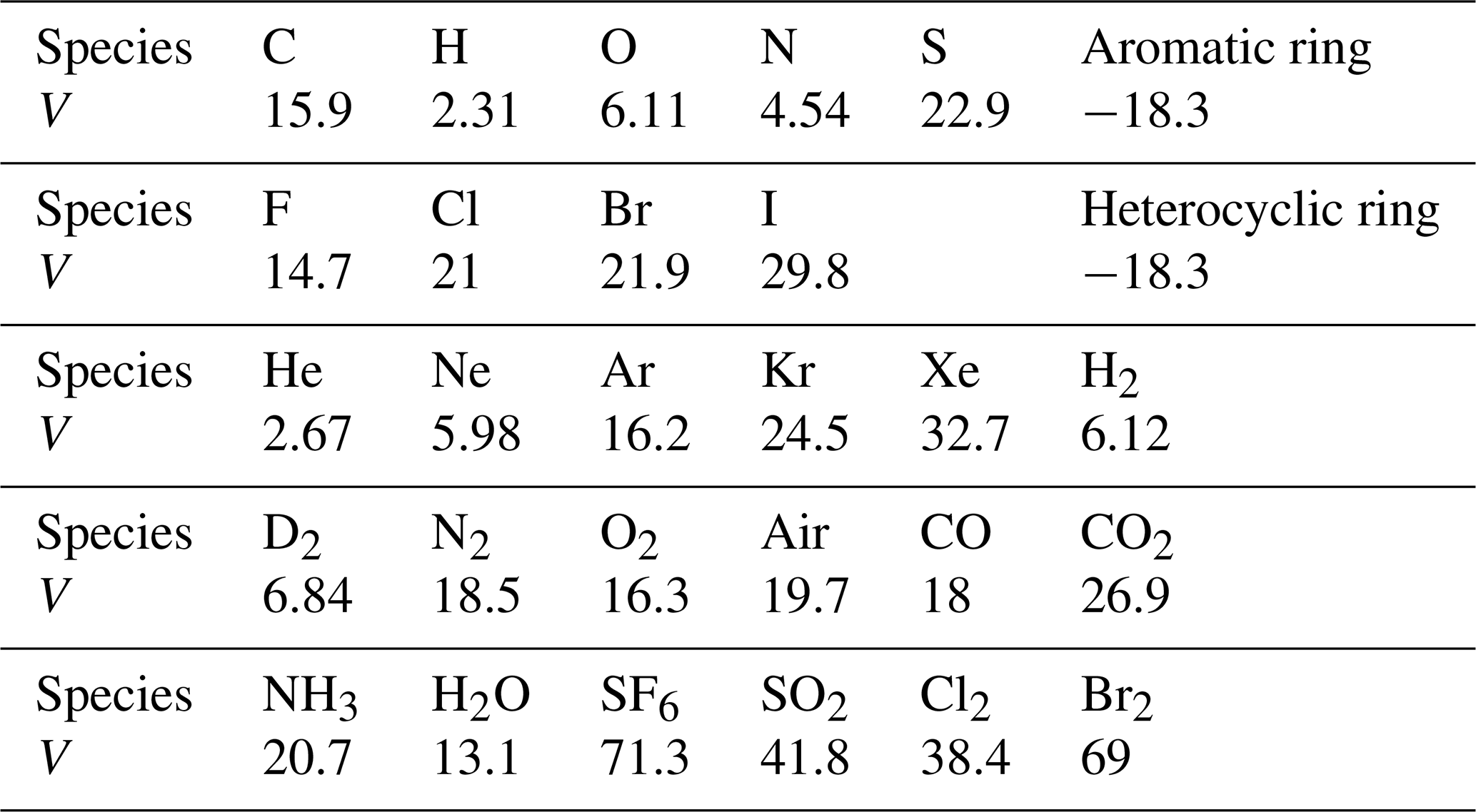
Therefore, an approximation for the mass diffusivity coefficient of phenol at 25 °C in nitrogen gas is calculated via Fuller’s method as:

$$\begin{array}{}\text{(B2)}& \begin{array}{rl}\mathcal{D}\left({\mathrm{C}}_{\mathrm{6}}{\mathrm{H}}_{\mathrm{6}}\mathrm{O},{\mathrm{N}}_{\mathrm{2}}\right)& ={\displaystyle \frac{\mathrm{1.0868}\cdot {\mathrm{298}}^{\mathrm{1.75}}}{\mathrm{760}\sqrt{\mathrm{43.17}}{\left(\sqrt[\mathrm{3}]{\mathrm{97.07}}+\sqrt[\mathrm{3}]{\mathrm{18.5}}\right)}^{\mathrm{2}}}}\\ & =\mathrm{0.0887}{\mathrm{cm}}^{\mathrm{2}}{\mathrm{s}}^{-\mathrm{1}}\end{array}\end{array}$$

Appendix C: Saturation vapour pressure via Clausius–Clayperon equation

If a value for the saturation vapour pressure of a species cannot be found in thermodynamic tables, it can be estimated using the Clausius–Clayperon equation and data from the Royal Society of Chemistry's Chemspider database to estimate saturation vapour pressures using the following equation (Pence and Williams, 2010):

$$\begin{array}{}\text{(C1)}& p\left(T\right)=p_{\mathrm{ref}}\exp \left(-{\displaystyle \frac{L_v}{R}}\left({\displaystyle \frac{\mathrm{1}}{T}}-{\displaystyle \frac{\mathrm{1}}{T_{\mathrm{ref}}}}\right)\right),\end{array}$$

where L_v is the latent heat of vaporization, R is the universal gas constant, and the subscript “ref” stands for a reference value (e.g. the values taken at room temperature). All of these values can be obtained from databases found on Chemspider (Pence and Williams, 2010).

Appendix D: Diffuser cartridge and nebulizer dimensions

The dimensions of the diffuser cartridge are shown in Fig. D1. The annular area of the nebulizer tip is 1.62 × 10⁻⁸ m².

Figure D1 Diffuser cartridge schematic diagram: (a) counter-hole, (b) hole, (c) O-ring spacer, (d) cross-sectional diagram of assembled diffuser cartridge.

Appendix E: Speed of sound and temperature at the atomizer tip

The choking pressure ratio for air is around a factor of 2, which is easily reached for the conditions through the nebulizer. The corresponding critical temperatures and velocities are given as follows:

$$\begin{array}{}\text{(E1)}& {\displaystyle }{T}^{*}=T_{\mathrm{0}}{\displaystyle \frac{\mathrm{2}}{\mathrm{1}+\mathit{\gamma }}}=\mathrm{244.16}\mathrm{K},\text{(E2)}& {\displaystyle }u=c^{*}=\sqrt{{\displaystyle \frac{\mathit{\gamma }R{T}^{*}}{M_{\mathrm{r}}}}}=\mathrm{318.6}\mathrm{m}{\mathrm{s}}^{-\mathrm{1}}.\end{array}$$

Appendix F: Approximating constrictions as porous media

Certain sections in the ELSD geometry contain constrictions which will affect the flow velocity and streamlines. Some of these sections, such as the diffuser cartridge, have manufacturing regulations that ensure an exact replica of the design, and its effect on the flow field is recreated every run; thus, the section can be made into a 3D geometry file and used in CFD. However, some design elements, such as the steel meshing that is placed on the waste collection pipe of the ELSD, does not have a set configuration when put in place, meaning that, although its effect on the flow field may be approximately equal across different devices, it is difficult to incorporate an exact 3D model of this part.

Figure F1 Diagram showing the positioning of the steel mesh in the ELSD waste collection pipe.

As such, the effect of the steel mesh on the flow may be approximated by treating it as a porous medium. The flow velocity across a porous medium can be approximated by using Darcy's Law:

$$\begin{array}{}\text{(F1)}& u_{\sup }=-{\displaystyle \frac{k\mathrm{\Delta }P}{{\mathit{\mu }}_{\mathrm{g}}L}},\end{array}$$

where u_sup is the superficial velocity of the fluid through the porous medium, k is the porous medium's permeability, ΔP is the pressure difference across the porous medium, μ_g is the dynamic viscosity of the fluid, and L is the length of the porous medium.

Ansys Fluent treats porous media through an extension of Darcy's Law:

$$\begin{array}{}\text{(F2)}& -\mathrm{\nabla }p=\mathit{\alpha }{\mathit{\mu }}_{\mathrm{g}}\mathit{v}+\mathit{\beta }{\mathit{\rho }}_{\mathrm{g}}\left|\mathit{v}\right|\mathit{v},\end{array}$$

where ∇p is the pressure gradient across the porous medium; v is the velocity vector across the porous medium; and the constants α and β are the coefficient of viscous flow resistance (which is the inverse of permeability, $\mathrm{1}/k$) and the coefficient of inertial flow resistance, respectively. Both constants can be obtained by using a method where the constriction is isolated in a pipe, whilst the pressure difference and flow velocity are varied according to the following relationship (Geertsma, 1974; Shkolnikov et al., 2010):

$$\begin{array}{}\text{(F3)}& -{\displaystyle \frac{p_L^{\mathrm{2}}-p_{\mathrm{0}}^{\mathrm{2}}}{\mathrm{2}Lc\mathit{\rho }{u}_{\sup }{\mathit{\mu }}_{\mathrm{g}}}}=\mathit{\alpha }+\mathit{\beta }{\displaystyle \frac{\mathit{\rho }{u}_{\sup }}{{\mathit{\mu }}_{\mathrm{g}}}},\end{array}$$

where the constants α and β were experimentally found to be 1.54 × 10⁷ and 411 m⁻¹, respectively, whilst the porosity of the steel mesh was determined to be 0.953.

Appendix G: Discrete phase model

A DPM is implemented in the CFD calculations in order to introduce the aerosol particles and to calculate their trajectories. In this study, the particles were treated as inert pure water droplets. A node-based averaging function is applied in order to try reduce the error associated with particle sizes which are of the same order of magnitude as the cell size. The effects of discrete phase sources on the gas phase are distributed between the cell which contains the centre of the droplet and its neighbouring cells. The DPM profile has an inverse dependence on the distance between the droplet centre and the node of each cell:

$$\begin{array}{}\text{(G1)}& {\displaystyle \frac{{\mathit{\phi }}_{p,n}}{{\mathit{\phi }}_{\mathrm{p}}}}={\displaystyle \frac{\mathrm{1}/\left|{\mathit{r}}_n-{\mathit{r}}_{\mathrm{p}}\right|}{\mathrm{1}/{\sum }_m\left|{\mathit{r}}_m-{\mathit{r}}_{\mathrm{p}}\right|}},\end{array}$$

where φ_p,n is a the source quantity released from the droplet source p into node n; φ_p is the total value of the source quantity from centre p; while r_p, r_m and r_n are the position vectors of the droplet centre for source p, the node m and the node n, respectively.

Appendix H: Governing equations

The gas-phase conservation equation is given for each gas species, i, as follows:

$$\begin{array}{}\text{(H1)}& {\displaystyle \frac{\partial \left(\mathit{\rho }{Y}_i\right)}{\partial t}}+\mathrm{\nabla }\cdot \left(\mathit{\rho }{Y}_i\mathbf{v}\right)=-\mathrm{\nabla }\cdot {\mathbf{J}}_i+M_i+S_i,\end{array}$$

where M_i is the net production rate of species i; S_i is the source term for species i from droplets; and J_i is the diffusion flux of species i and is calculated as

$$\begin{array}{}\text{(H2)}& {\mathbf{J}}_i=-\mathit{\rho }{\mathcal{D}}_i\mathrm{\nabla }{Y}_i-{\mathcal{D}}_i-{\mathit{\alpha }}_i{\displaystyle \frac{\mathrm{\nabla }T}{T}},\end{array}$$

where 𝒟 is mass diffusivity and α is the thermal diffusivity. The gas momentum equation is solved via (Prosperetti and Tryggvason, 2009)

$$\begin{array}{}\text{(H3)}& {\displaystyle \frac{\partial }{\partial t}}\left(\mathit{\rho }\mathbf{v}\right)+\mathrm{\nabla }\cdot \left(\mathit{\rho }\mathbf{vv}\right)=-\mathrm{\nabla }p+\mathrm{\nabla }\cdot \mathit{\tau }+\mathit{\rho }\mathbf{g}+{\mathbf{F}}_{\mathrm{e}},\end{array}$$

where τ is the stress tensor, and F_e denotes external body forces, in this case the drag force related to the momentum change between droplets and the gas flow, which is expressed as

$$\begin{array}{}\text{(H4)}& {\mathbf{F}}_{\mathrm{e}}=\sum _k\left({\displaystyle \frac{\mathrm{18}\mathit{\mu }\mathit{Re}{C}_{\mathrm{D}}}{\mathrm{24}{\mathit{\rho }}_k{d}_k^{\mathrm{2}}}}\right)\left(u_k-u_{\mathrm{g}}\right)m_k,\end{array}$$

where C_D is the drag coefficient, approximated as follows (Morsi and Alexander, 1972):

$$\begin{array}{}\text{(H5)}& C_{\mathrm{D}}={\mathit{\alpha }}_{\mathrm{1}}+{\displaystyle \frac{{\mathit{\alpha }}_{\mathrm{2}}}{\mathit{Re}}}+{\displaystyle \frac{{\mathit{\alpha }}_{\mathrm{3}}}{{\mathit{Re}}^{\mathrm{2}}}},\end{array}$$

where the values of α₁, α₂ and α₃ differ over eight ranges of values depending on the Reynolds Number (Morsi and Alexander, 1972).

Appendix I: Thermophoresis and diffusive losses

The thermal force imparted on a particle, causing it to move from a region of high temperature towards a region of low temperature, is given as follows (Hinds and Zhu, 2022):

$$\begin{array}{}\text{(I1)}& F_{\mathrm{th}}=\left\{\begin{array}{ll}\frac{-p\mathit{\lambda }{d}_{\mathrm{p}}^{\mathrm{2}}\mathrm{\nabla }T}{T}& \text{for}{d}_{\mathrm{p}}<\mathit{\lambda },\\ \frac{-\mathrm{9}\mathit{\pi }{d}_{\mathrm{p}}{\mathit{\mu }}_{\mathrm{g}}^{\mathrm{2}}H\mathrm{\nabla }T}{\mathrm{2}{\mathit{\rho }}_{\mathrm{g}}T}& \text{for}{d}_{\mathrm{p}}>\mathit{\lambda },\end{array}\right.\end{array}$$

where p is the gas pressure, and λ is the gas mean free path. The coefficient H includes the effect of a temperature gradient inside of a particle, while ∇T is the overall temperature gradient without considering the particle. The minus sign is required to indicate the direction of the force towards decreasing temperature.

The coefficient H is given by the following:

$$\begin{array}{}\text{(I2)}& H=\left({\displaystyle \frac{\mathrm{1}}{\mathrm{1}+\mathrm{6}\mathit{\lambda }/d_{\mathrm{p}}}}\right)\left({\displaystyle \frac{k_{\mathrm{a}}/k_{\mathrm{p}}+\mathrm{4.4}\mathit{\lambda }/d_{\mathrm{p}}}{\mathrm{1}+\mathrm{2}{k}_{\mathrm{a}}/k_{\mathrm{p}}+\mathrm{8.8}\mathit{\lambda }/d_{\mathrm{p}}}}\right),\end{array}$$

where k_a and k_p are the thermal conductivities of air and the particle, respectively.

Hinds and Zhu (2022) give the thermophoretic velocity of a particle as follows:

$$\begin{array}{}\text{(I3)}& V_{\mathrm{th}}=\left\{\begin{array}{ll}\frac{-\mathrm{0.55}{\mathit{\mu }}_{\mathrm{g}}\mathrm{\nabla }T}{{\mathit{\rho }}_{\mathrm{g}}T}& \text{for}{d}_{\mathrm{p}}<\mathit{\lambda },\\ \frac{-\mathrm{3}{\mathit{\mu }}_{\mathrm{g}}{\text{C}}_{\mathrm{c}}H\mathrm{\nabla }T}{\mathrm{2}{\mathit{\rho }}_{\mathrm{g}}T}& \text{for}{d}_{\mathrm{p}}>\mathit{\lambda },\end{array}\right.\end{array}$$

where C_c is the Cunningham slip correction factor. The deposition velocity of a particle due to diffusive forces is given by Hinds and Zhu (2022) as follows:

$$\begin{array}{}\text{(I4)}& V_{\mathrm{dif}}={\displaystyle \frac{\mathrm{0.04}{u}_{\mathrm{g}}}{{\mathit{Re}}^{\frac{\mathrm{1}}{\mathrm{4}}}}}{\left({\displaystyle \frac{{\mathit{\rho }}_{\mathrm{g}}{\mathcal{D}}_{\mathrm{p}}}{{\mathit{\mu }}_{\mathrm{g}}}}\right)}^{\frac{\mathrm{2}}{\mathrm{3}}},\end{array}$$

where 𝒟_p represents the diffusivity of the aerosol particle in the fluid, as given by the Stokes–Einstein equation (Hinds and Zhu, 2022).

$$\begin{array}{}\text{(I5)}& {\mathcal{D}}_{\mathrm{p}}={\displaystyle \frac{k_{B}T{\text{C}}_{\mathrm{c}}}{\mathrm{3}\mathit{\pi }{\mathit{\mu }}_{\mathrm{g}}{d}_{\mathrm{p}}}}\end{array}$$

Thus, because the diffusive forces affecting the aerosol act outwards towards the hot walls and the thermophoretic forces direct the aerosol away from the hot walls, a deposition velocity can be defined as the difference between the two:

$$\begin{array}{}\text{(I6)}& V_{\mathrm{dep}}=V_{\mathrm{dif}}-V_{\mathrm{th}}.\end{array}$$

Finally, the overall penetration through a tube of length L and diameter d_L subject to losses to the walls by diffusion or inertia is given by Hinds and Zhu (2022) as follows:

$$\begin{array}{}\text{(I7)}& \mathcal{P}=\exp \left({\displaystyle \frac{-\mathrm{4}{V}_{\mathrm{dep}}L}{d_L{u}_{\mathrm{g}}}}\right).\end{array}$$

Figure I1 Calculated deposition velocity for a range of evaporator tube temperatures and particle diameters.

The effects of thermophoresis and diffusion were not found to be significant for the current problem, where the leading-order terms are convection and evaporation.

Appendix J: Light scattering signal using Mie theory

The MATLAB-based model simulating the ELSD signal response within this work, described in Sect. 3.5, uses MATLAB functions which were based on the work of Mätzler (2002). These scripts were written using equations for single spherical particle scattering as given by Mie theory (Huber and Frost, 1998; van de Hulst, 1981) based on the following assumptions:

• Particles are spherical.

• Particle refractive index, which may be complex (m = m₁+im₂), is homogeneous across the particle and is different to that of the surrounding medium.

• Incident light is a plane wave.

• Incident light is a travelling wave (i.e. field amplitudes are time harmonic).

• Incident light is monochromatic.

The light scattering size parameter, α = $\frac{\mathrm{2}\mathit{\pi }{r}_{\mathrm{p}}}{\mathit{\lambda }}$, characterizes the light scattering regime in which the particle belongs and is defined, where r_p is the particle radius, and λ is the wavelength of incident light. The scattering angle is given by θ, and the product between the particle refractive index m and the size parameter is given by Z, Z = αm.

Mätzler (2002) discretizes the domain into N_max angular locations, such that

$$\begin{array}{}\text{(J1)}& N_{max}=\mathtt{\text{ceil}}\left[\mathrm{2}+\mathit{\alpha }+{\mathit{\alpha }}^{\frac{\mathrm{1}}{\mathrm{3}}}\right],\end{array}$$

where ceil represents the rounding function in order to output an integer. The vectors N and ν of natural numbers are defined as follows:

$$\begin{array}{}\text{(J2)}& {\displaystyle }\mathit{N}=\left(\mathrm{1},\mathrm{\dots },N_{max}\right)\text{(J3)}& {\displaystyle }\mathit{\nu }=\mathit{N}+{\displaystyle \frac{\mathrm{1}}{\mathrm{2}}}.\end{array}$$

J1 Bessel functions

Bessel functions of the first kind and second kind, denoted by 𝒥 and 𝒴, respectively, are given by

$$\begin{array}{}\text{(J4)}& {\displaystyle }{\mathcal{J}}_A\left(B\right)=\sum _{k=\mathrm{0}}^{\mathrm{\infty }}\left({\displaystyle \frac{(-\mathrm{1}{)}^k}{k\mathrm{!}\mathrm{\Gamma }(k+A+\mathrm{1})}}{\left({\displaystyle \frac{B}{\mathrm{2}}}\right)}^{\mathrm{2}k+A}\right),\text{(J5)}& {\displaystyle }{\mathcal{Y}}_A\left(B\right)={\displaystyle \frac{{\mathcal{J}}_A\left(B\right)\cos \left(A\mathit{\pi }\right)-{\mathcal{J}}_{-A}\left(B\right)}{\sin \left(A\mathit{\pi }\right)}}.\end{array}$$

Vectors are calculated using Bessel functions for each element in the vector ν:

$$\begin{array}{}\text{(J6)}& {\displaystyle }{\mathit{b}}_{\mathit{\alpha }}=\sqrt{{\displaystyle \frac{\mathit{\pi }}{\mathrm{2}\mathit{\alpha }}}}{\mathcal{J}}_{\mathit{\nu }}\left(\mathit{\alpha }\right),\text{(J7)}& {\displaystyle }{\mathit{b}}_Z=\sqrt{{\displaystyle \frac{\mathit{\pi }}{\mathrm{2}Z}}}{\mathcal{J}}_{\mathit{\nu }}\left(Z\right),\text{(J8)}& {\displaystyle }{\mathit{y}}_{\mathit{\alpha }}=\sqrt{{\displaystyle \frac{\mathit{\pi }}{\mathrm{2}\mathit{\alpha }}}}{\mathcal{Y}}_{\mathit{\nu }}\left(\mathit{\alpha }\right),\text{(J9)}& {\displaystyle }{\mathit{h}}_{\mathit{\alpha }}={\mathit{b}}_{\mathit{\alpha }}+{\mathit{y}}_{\mathit{\alpha }}+i,\end{array}$$

where the vector h is vector which is analogous to a modified Hankel function of the first kind. From these, the following series of vectors are also constructed:

$$\begin{array}{}\text{(J10)}& {\displaystyle }{\mathit{B}}_{\mathit{\alpha }}=\left({\displaystyle \frac{\sin \left(\mathit{\alpha }\right)}{\mathit{\alpha }}},b_{{\mathit{\alpha }}_{\mathrm{1}}},\mathrm{\dots },b_{{\mathit{\alpha }}_{N_{max}-\mathrm{1}}}\right),\text{(J11)}& {\displaystyle }{\mathit{B}}_Z=\left({\displaystyle \frac{\sin \left(Z\right)}{Z}},b_{Z_{\mathrm{1}}},\mathrm{\dots },b_{Z_{N_{max}-\mathrm{1}}}\right),\text{(J12)}& {\displaystyle }{\mathit{Y}}_{\mathit{\alpha }}=\left({\displaystyle \frac{-\cos \left(\mathit{\alpha }\right)}{\mathit{\alpha }}},y_{{\mathit{\alpha }}_{\mathrm{1}}},\mathrm{\dots },y_{{\mathit{\alpha }}_{N_{max}-\mathrm{1}}}\right),\text{(J13)}& {\displaystyle }{\mathit{H}}_{\mathit{\alpha }}={\mathit{B}}_{\mathit{\alpha }}+{\mathit{Y}}_{\mathit{\alpha }}+i.\end{array}$$

The vectors constructed above are used to compute the following using element-wise vector multiplication, which is denoted by the Hadamard product (⊙):

$$\begin{array}{}\text{(J14)}& {\displaystyle }{\mathit{A}}_{\mathit{\alpha }}=\mathit{\alpha }{\mathit{B}}_{\mathit{\alpha }}-\mathit{N}\odot {\mathit{b}}_{\mathit{\alpha }},\text{(J15)}& {\displaystyle }{\mathit{A}}_Z=Z{\mathit{B}}_Z-\mathit{N}\odot {\mathit{b}}_Z,\text{(J16)}& {\displaystyle }{\mathcal{H}}_{\mathit{\alpha }}=\mathit{\alpha }{\mathit{H}}_{\mathit{\alpha }}-\mathit{N}\odot {\mathit{h}}_{\mathit{\alpha }}.\end{array}$$

Finally, the vectors a_n, b_n, c_n and d_n are calculated using element-wise vector multiplication (denoted by the Hadamard product, as above) and element-wise division (Hadamard division, denoted by ⊘).

$$\begin{array}{}\text{(J17)}& {\displaystyle }\begin{array}{rl}{a}_n=& \left(\left|\right|m|{|}^{\mathrm{2}}\odot {\mathit{b}}_z\odot \left({\mathit{A}}_{\mathit{\alpha }}-{\mathit{b}}_{\mathit{\alpha }}\right)\odot {\mathit{A}}_Z\right)\\ & \oslash \left(\left|\right|m|{|}^{\mathrm{2}}\odot {\mathit{b}}_Z\odot \left({\mathcal{H}}_{\mathit{\alpha }}-{\mathit{h}}_{\mathit{\alpha }}\right)\odot {\mathit{A}}_Z\right)\end{array}\text{(J18)}& {\displaystyle }{b}_n=\left({\mathit{b}}_Z\odot \left({\mathit{A}}_{\mathit{\alpha }}-{\mathit{b}}_{\mathit{\alpha }}\right)\odot {\mathit{A}}_Z\right)\oslash \left({\mathit{b}}_Z\odot \left({\mathcal{H}}_{\mathit{\alpha }}-{\mathit{h}}_{\mathit{\alpha }}\right)\odot {\mathit{A}}_Z\right)\text{(J19)}& {\displaystyle }{c}_n=\left({\mathit{b}}_{\mathit{\alpha }}\odot \left({\mathcal{H}}_{\mathit{\alpha }}-{\mathit{h}}_{\mathit{\alpha }}\right)\odot {\mathit{A}}_{\mathit{\alpha }}\right)\oslash \left({\mathit{b}}_Z\odot \left({\mathcal{H}}_{\mathit{\alpha }}-{\mathit{h}}_{\mathit{\alpha }}\right)\odot {\mathit{A}}_Z\right)\text{(J20)}& {\displaystyle }\begin{array}{rl}{d}_n=& m\odot \left({\mathit{b}}_{\mathit{\alpha }}\odot \left({\mathcal{H}}_{\mathit{\alpha }}-{\mathit{h}}_{\mathit{\alpha }}\right)\odot {\mathit{A}}_{\mathit{\alpha }}\right)\\ & \oslash \left(\left|\right|m|{|}^{\mathrm{2}}\odot {\mathit{b}}_Z\odot \left({\mathcal{H}}_{\mathit{\alpha }}-{\mathit{h}}_{\mathit{\alpha }}\right)\odot {\mathit{A}}_Z\right)\end{array}\end{array}$$

J2 Angular functions

The angular scattering functions, p and t, are defined as a sequence, forming a vector of length N_max.

The first two terms of p and t, are given as follows:

$$\begin{array}{}\text{(J21)}& {\displaystyle }{p}_{\mathrm{1}}=\mathrm{1},\text{(J22)}& {\displaystyle }{t}_{\mathrm{1}}=\cos \left(\mathit{\theta }\right),\text{(J23)}& {\displaystyle }{p}_{\mathrm{2}}=\mathrm{3}\cos \left(\mathit{\theta }\right),\text{(J24)}& {\displaystyle }{t}_{\mathrm{2}}=\mathrm{3}\cos \left(\mathrm{2}\mathit{\theta }\right).\end{array}$$

From k = 3 to k = N_max, p and t are defined by the following sequences:

$$\begin{array}{}\text{(J25)}& {\displaystyle }{p}_k=\left({\displaystyle \frac{\mathrm{2}k-\mathrm{1}}{k-\mathrm{1}}}\right)p_{k-\mathrm{1}}\cos \left(\mathit{\theta }\right)-\left({\displaystyle \frac{k}{k-\mathrm{1}}}\right)p_{k-\mathrm{2}},\text{(J26)}& {\displaystyle }{t}_k=k\cos \left(\mathit{\theta }\right)p_k-(k+\mathrm{1})p_{k-\mathrm{1}}.\end{array}$$

The sequence elements for p and t are gathered to construct the vectors p and t. Finally, the modified angular function vectors 𝓟 and 𝓣 are constructed via the following element-wise vector multiplication:

$$\begin{array}{}\text{(J27)}& {\displaystyle }\mathcal{P}=\mathcal{N}\odot \mathit{p},\text{(J28)}& {\displaystyle }\mathcal{T}=\mathcal{N}\odot \mathit{t},\end{array}$$

where 𝓝 is the vector

$$\begin{array}{}\text{(J29)}& \mathcal{N}=\left(\mathrm{2}\mathit{N}+\mathrm{1}\right)\oslash \left(\mathit{N}\odot (\mathit{N}+\mathrm{1})\right).\end{array}$$

J3 Determination of light scattering intensity

The use of the vector parameters obtained via the Bessel functions and angular functions allows for the calculation of the parameters in the scattering matrix of the particle, S₁ and S₂:

$$\begin{array}{}\text{(J30)}& {\displaystyle }{S}_{\mathrm{1}}={\mathit{a}}_n{\mathcal{P}}^{\text{T}}+{\mathit{b}}_n{\mathcal{T}}^{\text{T}},\text{(J31)}& {\displaystyle }{S}_{\mathrm{2}}={\mathit{a}}_n{\mathcal{T}}^{\text{T}}+{\mathit{b}}_n{\mathcal{P}}^{\text{T}}.\end{array}$$

The scattering matrix parameters determine the relation between incident, I₀, and scattered field, I, amplitudes via the following equation:

$$\begin{array}{}\text{(J32)}& {\displaystyle \frac{I}{I_{\mathrm{0}}}}={\displaystyle \frac{{\mathit{\lambda }}^{\mathrm{2}}}{\mathrm{8}{\mathit{\pi }}^{\mathrm{2}}{R}^{\mathrm{2}}}}\left(\left|\right|S_{\mathrm{1}}|{|}^{\mathrm{2}}+|\left|S_{\mathrm{2}}\right|{|}^{\mathrm{2}}\right),\end{array}$$

where R is the distance of the laser source to the scattering particle, and the squared magnitudes of the scattering matrix parameters, $\left|\right|S_{\mathrm{1}}|{|}^{\mathrm{2}}$ and $\left|\right|S_{\mathrm{2}}|{|}^{\mathrm{2}}$, represent the intensity of perpendicular and parallel scattered light, respectively.