Dispersion normalisation method for improved long-term trend evaluation: heavy metals in ambient air in the Czech Republic, Central Europe (2010–2021)

Long-term trends in atmospheric concentrations of heavy metals subject to legislative immission limits (As, Cd, Pb, Ni) were evaluated at selected monitoring stations representing different environmental settings across the Czech Republic (in Central Europe) over 12 years. Dispersion normalisation was applied to reduce the influence of meteorological variability on measured concentrations and to assess the effectiveness of legislative emission control measures. The results demonstrated statistically significant decreasing trends (p < 0.001) across all station types and for all monitored heavy metals, aside from Ni at the industrial station, where no significant trend was detected. Furthermore, systematic differences between original and dispersion-normalised concentration data indicate that meteorological variability can, in some cases, mask actual emission levels, potentially leading to misinterpretation of air quality trends.

Dispersion normalisation proved to be a suitable method for long-term trend assessment and for quantifying the impact of regulatory measures on air quality. The method's key advantages include simplicity and the availability of input data required to calculate the ventilation coefficient (e.g. from ERA5).

1 Introduction

Heavy metal (HM) pollution remains a significant environmental issue due to its persistence in the environment and its harmful effects on human health and ecosystems, including toxicity and bioaccumulation in the human body (EEA, 2013; Mitra et al., 2022; Suvarapu and Baek, 2017). In the atmosphere, heavy metals are usually released in particulate form or become associated with aerosol particles after release, which may be inhaled and contribute to adverse health effects. These HM-polluted particles can also be deposited into soil and water, contributing to wider environmental contamination. The emission of HMs into the atmosphere is heavily associated with anthropogenic activities, including industry, transportation, and mining (Ma et al., 2024).

Despite reductions in emissions and ambient levels since the 1990s (EEA, 2024, 2025), HMs still require strict regulation as they do not degrade in nature (e.g. Ahmad et al., 2021; Briffa et al., 2020; Mitra et al., 2022). This need is reflected in regulations such as the Convention on Long-range Transboundary Air Pollution (CLRTAP) – Protocol on Heavy Metals, Directive 2004/107/EC, and Directive 2008/50/EC. The relevance of this issue is further underscored by EU Regulation 2023/915 on maximum levels of selected elemental contamination in food, including HMs, and Directive (EU) 2024/2881 on ambient air quality and cleaner air for Europe. In the Czech Republic, national law integrates these EU regulations and directives concerning HM emission and immission limits through Act no. 201/2012 Sb. The immission limits for selected HMs, such as arsenic (As, 6 ng m⁻³), cadmium (Cd, 5 ng m⁻³), lead (Pb, 500 ng m⁻³), and nickel (Ni, 20 ng m⁻³), have been established in the Czech Republic.

Consequently, air quality in this region has been steadily improving (Aas et al., 2024). Nevertheless, Central Europe remains one of the regions with the highest concentrations and deposition rates of HMs in Europe (Travnikov et al., 2020). Therefore, this study examines levels and trends in HM concentrations in relation to immission limits in the Czech Republic over the period 2010–2021. The analysis covers multiple types of environments and focuses on the effects of current regulatory measures. Dispersion normalisation is applied here for the first time in the context of HM assessment to reduce the influence of meteorological variability on observed concentrations and trends at air quality monitoring stations. To better understand these developments, this study addresses three main objectives.

The main objectives of the study are as follows:

1. Evaluate long-term trends in HM concentration at different types of monitoring stations in the Czech Republic.

2. Investigate the suitability of selected monitoring stations and establish a representative station group. A critical research question relates to whether a single monitoring station can be representative of the entire network or whether multiple stations are necessary to ensure data reliability. The study aims to identify potential methodological challenges and limitations associated with the selection and grouping of monitoring stations in the assessment of emission-related trends.

3. Examine the influence of meteorological variables on measured immission concentrations in relation to evaluating the effects of emission regulations. The study evaluates whether normalisation techniques constitute an appropriate methodological tool for isolating emission signals from meteorological influence. Specifically, the study focuses on dispersion normalisation using the ventilation coefficient. The differences between the original (HM_OR) and dispersion-normalised (HM_DN) HM concentration datasets are evaluated. The goal of this objective is to explore the potential masking of changes in emission signals due to meteorological effects.

2 Sources of HMs and emission structure in the Czech Republic

HMs, similarly to many other pollutants, are released into the atmosphere through natural and anthropogenic processes. Typical natural sources of the studied HMs are volcanic eruptions, soil erosion and soil dust, and wildfires (EEA, 2013; Tchounwou et al., 2012). The primary anthropogenic sources of As are metal smelters and fuel combustion (EEA, 2013) and the manufacturing of insecticides, herbicides, and similar inhibitors (Tchounwou et al., 2012). Cd emissions from anthropogenic sources mainly originate from the production of non-ferrous metals, stationary fossil fuel combustion, and waste incineration. Anthropogenic Pb emissions include traffic, fossil fuel combustion, waste incineration, and the production of non-ferrous metals. Another important source of Pb is the resuspension of road dust, especially applicable to locations affected by road traffic. The main source of anthropogenic Ni emissions is the combustion of oil (whether it be for heating, shipping, or power generation), mining, and waste incineration (EEA, 2013).

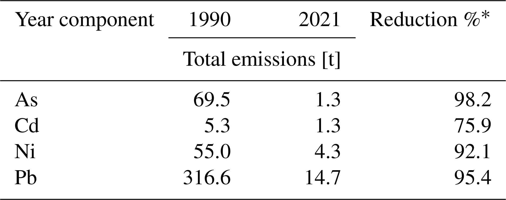
Between 1990 and 2021, emissions in the Czech Republic changed in terms of both magnitude and source structure. The most dramatic change was recorded for total As and Pb emissions, with As emissions dropping to 1.8 % of the 1990 value, i.e. by 98.2 %, and Pb emissions decreasing to 4.6 %, i.e. by 95.4 %. In contrast, Cd emissions declined to only 24 % of the 1990 value, i.e. by 76 % (Table 1). The change in source structure between 1990 and 2021 is also visible. While one of the main source sectors for almost all studied HMs was iron and steel production in 1990, in 2021, the most common emission source was public electricity and heat production. The restriction of Pb content in fuel is reflected by the lowering of the contribution of the Road Transport: Passenger Car section (Fig. 1). More detailed information is accessible in the reports provided by the Czech Hydrometeorological Institute (CHMI) and the Centre on Emission Inventories and Projections (CEIP) (CHMI, 2026a; CEIP, 2024). The described changes indicate that the restrictions under the CLRTAP and EU directives (mentioned in the introduction) helped lower HM concentrations and limited some sources.

Table 1 Overview of total emissions in 1990 and 2021 in the Czech Republic. The structure of emissions changed in response to technological developments and regulatory measures. Source: CEIP (2024).

^∗ Reduction relative to 1990 levels.

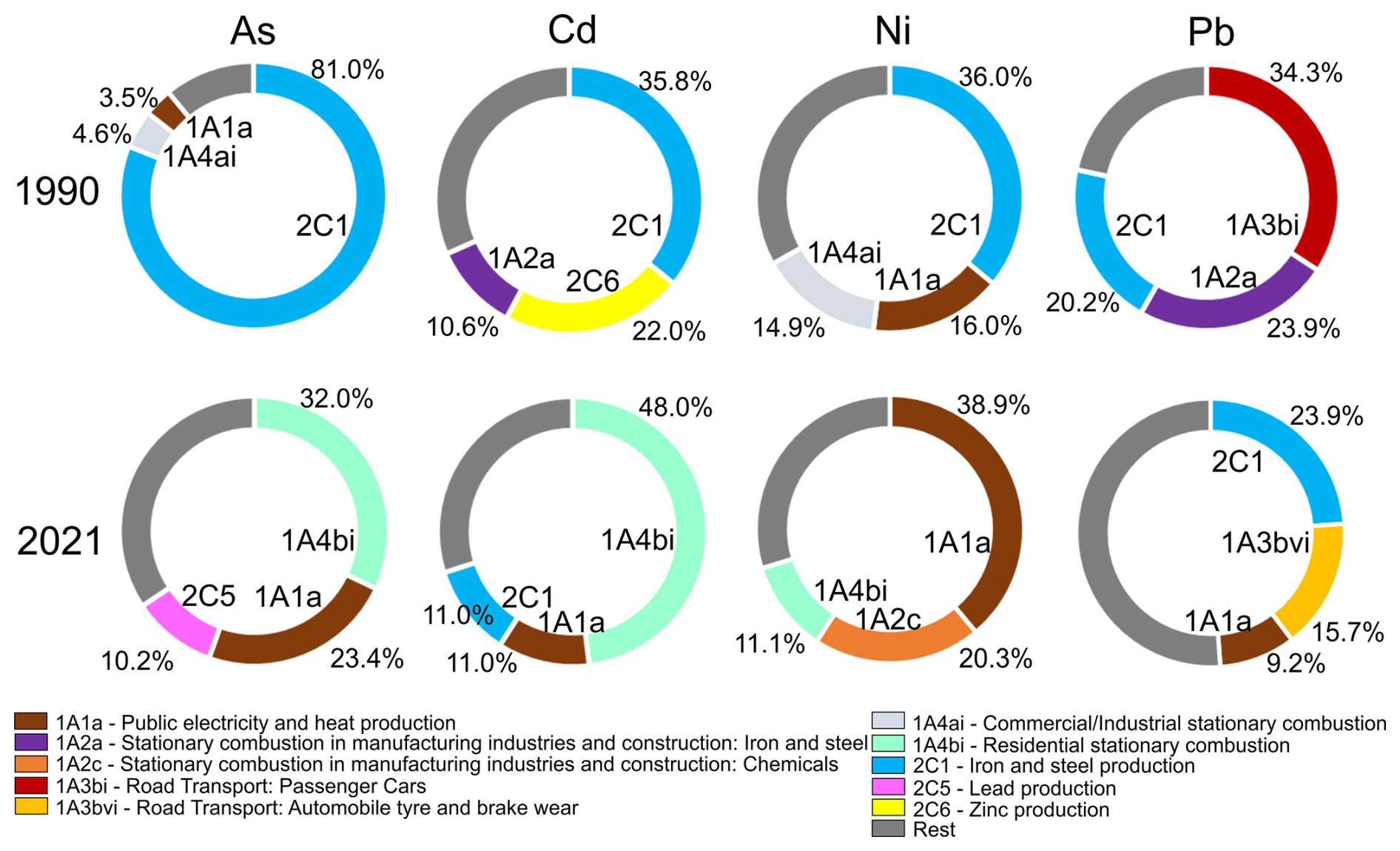
Figure 1 Structure of selected HM emission sources according to economic sectors in 1990 and 2021. Only the first three sectors are visualised; the other sources are in the “rest” category. Source: CEIP (2024).

A similar reduction in HM emissions observed in the Czech Republic was observed in the wider European region (Fig. S1 in the Supplement). Beyond domestic emission sources, transboundary transport should be considered to be a significant contributor to elevated HM concentrations. For instance, according to Travnikov et al. (2020), transboundary transport accounts for 7 %–99 % of Cd deposition from non-national sources in EMEP member countries.

3 Atmospheric boundary layer and ventilation coefficient

Meteorological conditions affect measured pollutant concentrations. Some meteorological parameters are spatially variable. Their involvement in calculating their influence on pollution concentration is complex and thus requires the use of similarly complex models (Gilliam et al., 2006; Williams, 2013; Zhang, 2019). To simplify calculations of the effect of meteorological conditions on pollutant concentrations, the ventilation coefficient (VC) parameter can be used. VC_i is defined as the product of atmospheric mixing layer height (MLH_i) and wind speed (u_i) at a particular height for the selected time interval (i) (e.g. Chen et al., 2022; Ferguson, 2001), as shown in Eq. (1):

$$\begin{array}{}\text{(1)}& {\mathrm{VC}}_i={\mathrm{MLH}}_i\times u_i.\end{array}$$

The relation between MLH, wind speed, and air pollution has been studied regularly (e.g. Ferguson, 2001; Holzworth, 1967; Iyer and Raj, 2013; Soleimanpour et al., 2023; Venegas and Mazzeo, 1999). An example of VC calculation can be found in Ashrafi et al. (2009) and Wu et al. (2023).

The variation in MLH is an important factor enabling the dilution of atmospheric pollution. MLH is a sublayer of the atmospheric boundary layer (ABL), reaching heights from ground level to hundreds of metres up to several kilometres. The dominant turbulent motion in this layer is driven by mechanical and thermal convection. Mechanical convection results from wind shear, while thermal convection is caused by the interaction of the Earth's surface with incoming solar radiation and the subsequent transfer of heat to a relatively cooler atmosphere (Berg et al., 2013; Stull, 2003, 2016). The diurnal height variation of the MLH and ABL is the result of meteorological factors, such as temperature, moisture, solar radiation, wind, and turbulence (Stull, 2016).

The VC and MLH parameters capture the evolution of key meteorological factors and can be used for dispersion normalisation. Accounting for meteorological conditions allows for more reliable evaluation and comparison of concentration data.

4 Methods

4.1 Selection of stations

HMs are regularly monitored within the National Air Quality Monitoring Network of the Czech Hydrometeorological Institute (CHMI). The monitoring network comprises over 30 manual stations and ca. 100 automatic air quality stations. However, for this study, only results from manual stations were deemed to be suitable. Further station selection was necessary to evaluate only measurements with complete data series for all selected parameters from 2010 to 2021. The data series had to fulfil the criteria outlined in Directive 2008/50/EC, Annex I, and Directive 2004/107/EC, Annex IV, for the presentation and validity of air pollution characteristics, i.e. a minimum of 90 % data coverage in an individual time period (CHMI, 2023). Under these rules, 16 stations across the Czech Republic were selected for this study (Fig. 2). These stations are located in different geographical areas.

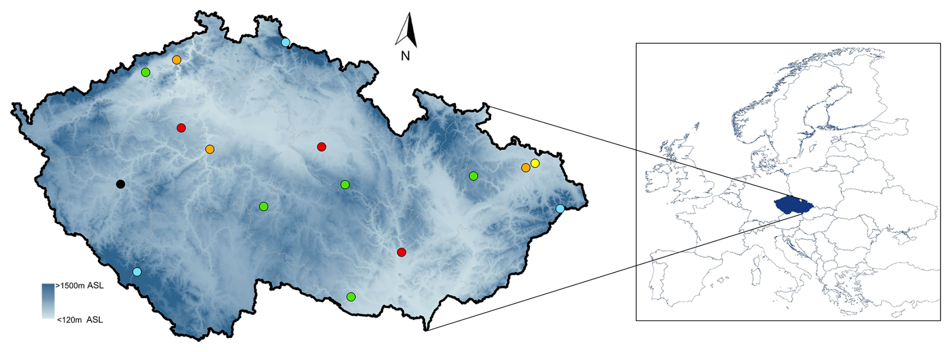
Figure 2 Spatial distribution of selected stations measuring HM in the period of 2010–2021 in the Czech Republic, Europe. Colours represent particular station types. Background rural mountain (BRM) stations are coloured light blue, background rural lowland (BRL) stations are in green, background urban (BU) stations are in red, background suburban (BS) stations are in orange, industrial (I) stations are in yellow, and traffic (T) stations are in black. ASL denotes metres above sea level. The map data were processed in ArcGIS software. Esri, 2018 | Powered by Esri.

Data were processed and evaluated in individual categories based on station type and altitude. The dataset was split into the following six categories: background rural mountain (BRM) stations, background rural lowland (BRL) stations, background urban (BU) stations, background suburban (BS) stations, industrial (I) stations, and traffic (T) stations. Basic characteristics are listed in Tables 2 and S1. The categorisation was done according to the EOI classification, which itself is based on Council Decision 97/101/EC (CHMI, 2023). Background rural stations were split into two subcategories based on station altitude. The border between lowland and mountain was set to 800 m a.s.l.

Table 2 Names and categories of selected stations.

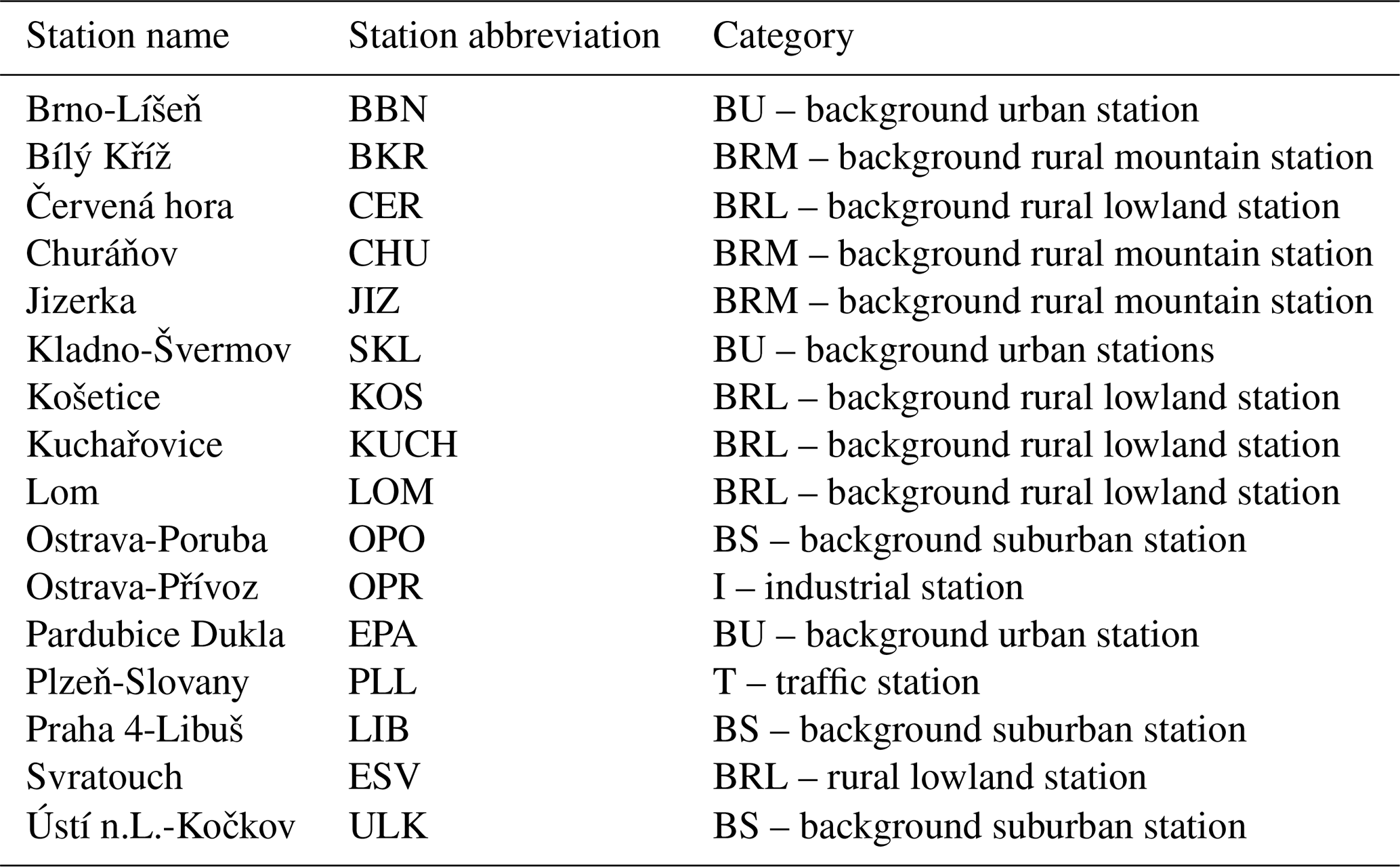
The main criterion for data processing was to maintain consistency and comparability within the time series; as such, the period 2019–2021 was chosen. Data after 2021 exhibited minor inconsistencies as technical issues with laboratory devices in 2022 and subsequent years resulted in temporary delays in analyses and produced gaps in the dataset.

4.2 Dispersion normalisation

The final dataset covers 12 years of data measured under different meteorological conditions. Therefore, correct evaluation requires data normalisation and the reduction in meteorological conditions. The reduction in meteorological influence was calculated according to a recently developed method intended for dispersion normalisation of Positive matrix factorisation analysis. This approach is widely used by the research community (e.g. Alfeus et al., 2024; Chen et al., 2022; Hopke, 2021; Mbengue et al., 2023; Wu et al., 2023; Yang et al., 2022). Dispersion normalisation concentration is calculated according to Eq. (2):

$$\begin{array}{}\text{(2)}& C_{\mathrm{DN}}=C_{\mathrm{OR}}\times {\displaystyle \frac{{\mathrm{VC}}_i}{\stackrel{\mathrm{‾}}{\mathrm{VC}}}},\end{array}$$

where C_DN denotes dispersion-normalised concentrations, C_OR is the measured (original) concentration, VC_i is the value of the ventilation coefficient, and $\stackrel{\mathrm{‾}}{\mathrm{VC}}$ is the averaged ventilation coefficient during the whole studied period.

The VC used in this study is taken from the Numerical Weather Prediction model's Aladin operation by CHMI. The calculation of VC for Czech conditions is based on the methodology listed in Ferguson (2001), with the thickness and average wind speed in the MLH being used (Škáchová, 2020; Škáchová and Keder, 2025).

4.3 Long-term trends

Trends in concentrations of individual components were evaluated using the Theil–Sen method (Carslaw and Ropkins, 2012; Sen, 1968; Theil, 1950), based on the non-parametric Mann–Kendall approach. This combination is an effective tool for analysing nonparametric data. In this analysis, the mean monthly values of the 75th or 95th percentiles of concentrations are considered (used, for example, in Lhotka et al., 2019).

The average slope of the trend, denoted by the T parameter, is calculated as follows:

$$\begin{array}{}\text{(3)}& T\left[\mathit{\%}\cdot {\mathrm{yr}}^{-\mathrm{1}}\right]=\mathrm{100}\cdot \left({\displaystyle \frac{C_{\mathrm{End}}}{C_{\mathrm{Start}}}}-\mathrm{1}\right)/N_{\mathrm{years}},\end{array}$$

where N_years is the number of years over which measurements were taken. C_End and C_Start represent the mean concentrations at the end and start of the measurement period, respectively.

The long-term trends were evaluated for both original and normalised data; however, the main focus was on the HM_DN results.

4.4 Sampling and analysis methods

The evaluated data were obtained from direct sampling at the selected stations. Each station measured the concentration of selected HMs in the PM₁₀ size fraction with a sequential sampling device (sequential sampler SQ47/50, Sven Leckel, Germany). The measurement was scheduled at a frequency of 1 × 2 d; the air was continuously sampled for 24 h starting at 00:00 UTC. Samples were, after exposure, analysed in accredited laboratories of the CHMI (according to the ČSN EN ISO/IEC 17025 standard) by inductively coupled plasma mass spectrometry (ICP-MS) (CHMI, 2023).

5 Results

5.1 Basic overview of HM concentrations measured at different station types

The HM concentrations varied according to station type. The lowest concentrations were observed at BRM stations, where median values reached 0.35 ng m⁻³ for As, 0.08 ng m⁻³ for Cd, 0.21 ng m⁻³ for Ni, and 2.1 ng m⁻³ for Pb. The second category exhibiting relatively low concentrations was represented by BRL stations, with median concentrations of 0.54 ng m⁻³ for As, 0.09 ng m⁻³ for Cd, 0.33 ng m⁻³ for Ni, and 2.57 ng m⁻³ for Pb. BS, BU, and T stations demonstrated comparable concentration levels across all evaluated HMs. Notably, As concentrations were elevated at BS, BU, and T station types, while Ni concentrations at T stations differed from those recorded at BU and BS locations. The median concentrations at BS, BU, and T stations were 0.79, 0.88, and 0.96 ng m⁻³ for As; 0.13, 0.14, and 0.14 ng m⁻³ for Cd; 0.48, 0.51, and 0.64 ng m⁻³ for Ni; and 4.70, 4.61, and 4.36 ng m⁻³ for Pb, respectively. The highest concentrations were measured at the I station type. The median As concentration reached 1.72 ng m⁻³, the Cd concentration reached 0.33 ng m⁻³, the Ni concentration reached 1.64 ng m⁻³, and the Pb concentration reached 14.90 ng m⁻³ (Fig. 3). A comparison between OR and DN results is visualised in Fig. S2.

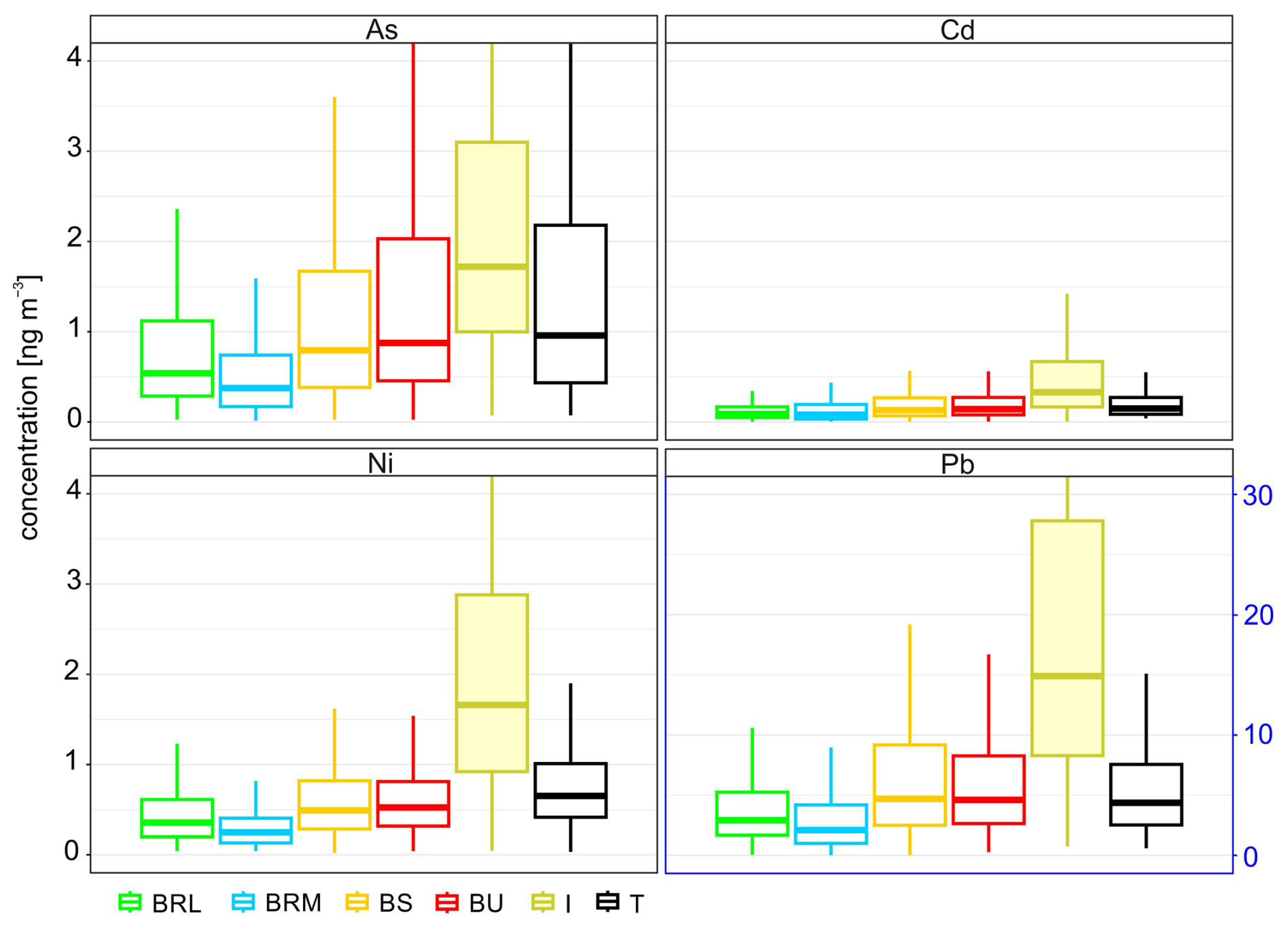
Figure 3 HM concentration overview at all station types, 2010–2021. Colours represent particular station types. Background rural mountain (BRM) stations are coloured light blue, background rural lowland (BRL) stations are in green, background urban (BU) stations are in red, background suburban (BS) stations are in orange, industrial (I) stations are in yellow, and traffic (T) stations are in black.

5.2 Integration of stations into groups

The stations were selected based on the availability of time series data and were grouped by type (according to EOI classification) and geographical location. The representativeness of each group was tested to assess eligibility and to confirm the relevance of the presented results. The data used for this verification were HM_DN to exclude meteorological variability at individual stations.

5.3 Correlation between individual stations and particular HM_DN

In order to compare results from individual stations, Spearman's correlation coefficient (R_s) values were calculated for HM_DN concentrations (Tables S2–S5). The correlation results were evaluated primarily for individual HM_DN using station pairs. Following Mukaka (2012) and Schober and Schwarte (2018), an R_s of 0.70 was chosen as the threshold for strong correlation. For As_DN, nine station pairs showed strong correlations, with the strongest being observed for LOM (R_s > 0.7 in three cases). For Cd, 22 station pairs demonstrated strong correlations, most often observed for LIB (R_s > 0.7 in six cases) and EPA (R_s > 0.7 in six cases) and for KOS and LOM (R_s > 0.7 in five cases). No station pairs with strong correlations were identified for Ni_DN (R_s 0.22–0.54). For Pb_DN, 19 pairs of stations showed strong correlations, most frequently involving KOS (R_s > 0.7 in five cases) and KUCH, ESV, LIB, BBN, and EPA (R_s > 0.7 in four cases each). These results suggest that Cd and Pb sources were relatively uniform across the Czech Republic and, by extension, Central Europe. In contrast, Ni concentrations and sources showed the most variability among all evaluated HM (consistently with Sect. 5.2.2 and 5.3.1). The lowest correlations (R_s < 0.6) were found for HM_DN concentrations at BRM stations. Dissimilar air masses impacting these locations on the Czech Republic's borders likely increase differences between stations compared to inland locations. Low R_s occurred frequently at the OPR industrial station, especially for As and Pb. These differences could be due to specific sources of As and Pb emissions in the Ostrava region, including steelworks, metallurgical plants, and mines.

The overall R_s pattern suggests that the relationship among station results is also influenced by mutual distance (Fig. 4). High R_s values (over 0.77) were found for OPR and OPO, BBN and KUCH, and LIB and SKL stations (except Ni_DN). When comparing correlations between all four studied HM_DN values at one station (Tables S6–S9), the highest correlation coefficients were found for Pb–Cd pairs (R_s = 0.72–0.94, median = 0.90) and Pb–As pairs (R_s = 0.70–0.87, median = 0.76), which could be related to their similar sources (industrial production, public energy, and/or residential heating). An exception is the correlation between Pb and Cd at JIZ (R_s = 0.62), where glass industry emissions influence Cd concentrations. Conversely, the lowest correlations were found for Ni–As and Ni–Pb pairs (R_s = 0.32–0.66), confirming the different trend in Ni concentrations compared to the remaining HMs.

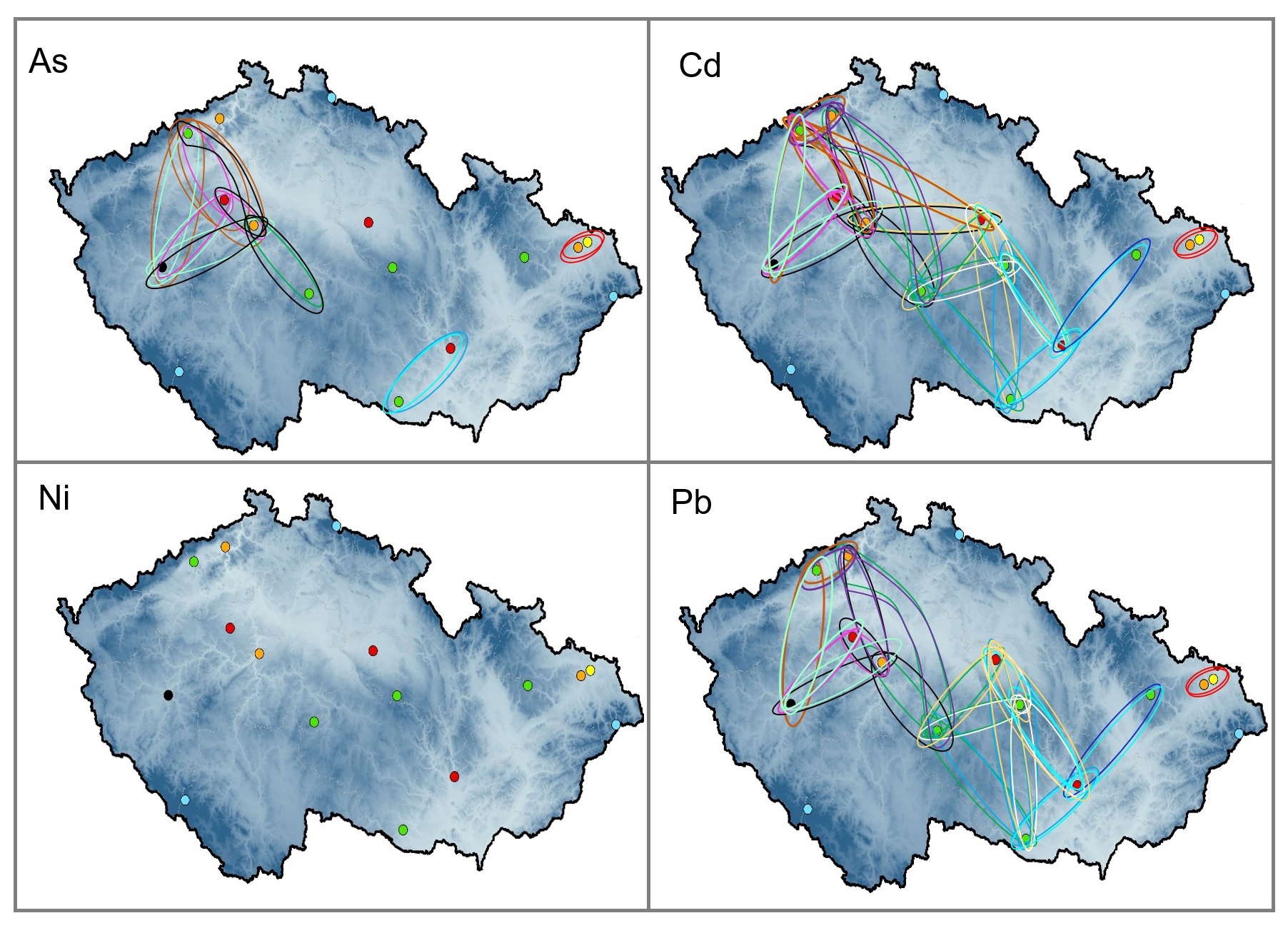
Figure 4 Spatial relationships among monitoring stations based on individual HM_DN correlations (R_s > 0.7). Coloured lines connect pairs of stations with strong correlations. Ellipses (circles) indicate spatial clusters of mutually correlated stations. Dot colours represent particular station type. Background rural mountain (BRM) stations are coloured light blue, background rural lowland (BRL) stations are in green, background urban (BU) stations are in red, background suburban (BS) stations are in orange, industrial (I) stations are in yellow, and traffic (T) stations are in black.

5.4 Verification using HM_DN long-term trends

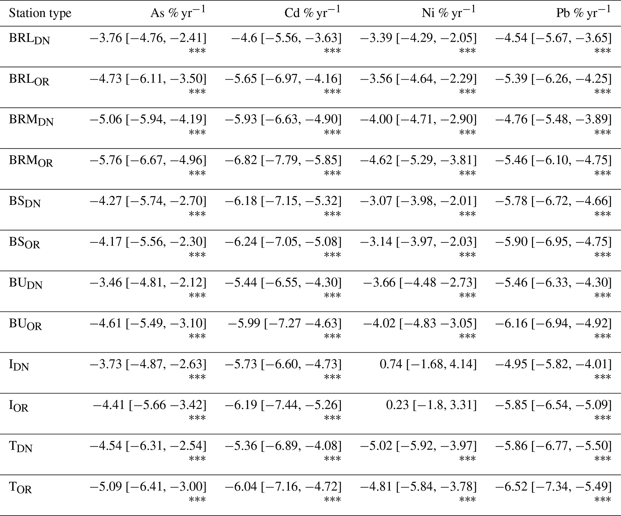
Each station and each HM was evaluated separately for long-term trend evolution (decreasing, increasing, or stable) and its statistical significance. The As_DN concentration trend was generally decreasing (p <  0.001) at all stations (Table 3), except for three stations. The LOM and ESV stations (both BRL station types) showed a slight decreasing trend with no statistical significance. The EPA station (BU) was characterised by a decreasing trend at the significance level p < 0.5 (Table S10). Results from the trend calculations for Cd_DN and Pb_DN concentrations showed a decreasing trend not only at the highest significance level across groups but also for all individual stations. The Ni_DN concentrations differed during the study period from those of the remaining HMs. The concentration trend analyses from individual stations are consistent with the overall trend analyses for groups. Note that BRM trend results show a significant trend (p < 0.001); however, two stations (BKR and CHU) showed a decreasing trend at a lower significance level (p < 0.01), with a similar result occurring for BS stations. The overall BS trend was at a significant level of p < 0.001; however, the ULK station indicated a decreasing trend at p <  0.01, and OPO showed a very slight decreasing tendency with no statistically significant trend. The industrial station OPR is represented by a slight increasing tendency with no statistically significant trend.

Table 3 Results of long-term trend analyses of HM concentrations for the grouped stations according to station type – EOI classification and altitude. Background rural lowland (BRL) stations, background rural mountain (BRM) stations, background suburban (BS) stations, background urban (BU) stations, industrial (I) stations, and traffic (T) stations. The overall trend is shown as a percentage increase or decrease per year, and the 95 % confidence intervals in the slope are listed in [% yr⁻¹]. Significance level: p <  0.001 = ${}^{\ast \ast \ast }$.

The individual HM concentration trend analyses confirmed that the data series from individual stations are suitable for group calculations and further evaluation. However, the individual behaviour of HM concentrations at a particular station should be taken into account in the data interpretation.

The statistical significance results were the same for the grouped HM_OR and HM_DN datasets. However, the percentage increase or decrease and confidence interval values were higher for HM_DN results (Table 3).

5.5 HM concentrations and patterns across station types

Across all investigated HMs, a divergence between OR and DN concentration datasets was observed, indicating meteorological influence on measured immission concentrations. The magnitude of differences varies among station types. A relatively stable response to meteorological conditions was observed at BRM stations (OR and DN difference interval of 19 %–51 %) and BRL stations (OR and DN divergence of 12 %–39 %). However, topography or microenvironmental characteristics were most evident at the T station type (OR–DN range: 8 %–52 %), where street canyon effects and building configurations likely modify meteorological influences on pollutant dispersion and accumulation. The OR–DN convergence over the years predominantly ranged from 7 % to 52 % across station types and the studied HM. The highest OR–DN convergence was observed in 2017 across the entire dataset (OR–DN range: 8 %–35 %), indicating good dispersion conditions reflected across all HM and environmental types, especially for Cd at BU and I stations and Pb at BU and T stations.

All station types exhibited statistically significant declines in As, Cd, Ni, and Pb (p < 0.001), providing clear evidence of the effectiveness of emission reduction policies. The consistency of these trends across rural, suburban, urban, industrial, and traffic environments highlights the regional-scale impact of legislative measures rather than isolated local improvements. Specific behaviour was recorded for Ni, where constant OR–DN divergence occurred at all station types. No trend was observed for the I station, which is an unusual pattern in the datasets studied.

5.6 Concentrations of As, Cd, Pb, and Ni at different station types

As showed statistically significant declines across all station types (p <  0.001), with annual reduction rates ranging from 3.45 % (BU) to 5.93 % (BRM). This consistent pattern suggests that the observed decrease is at least partly associated with legislative measures targeting As emissions. The highest As_DN concentrations were recorded at the I station (0.83–1.92 ng m⁻³), as expected, due to industry being the dominant source of As.

Differences between As_OR and As_DN (7 %–47 %) likely reflect not only episodic emission events but also the influence of meteorological conditions. A short-term increase in emission-related concentrations during 2011–2013 is more clearly captured in the dispersion-normalised data, particularly at T and I stations, where it is less apparent in the original time series due to meteorological variability. This effect can be observed in Fig. 5, where the DN data reveal a distinct, temporary deviation from the long-term trend, which is partially masked in the OR data.

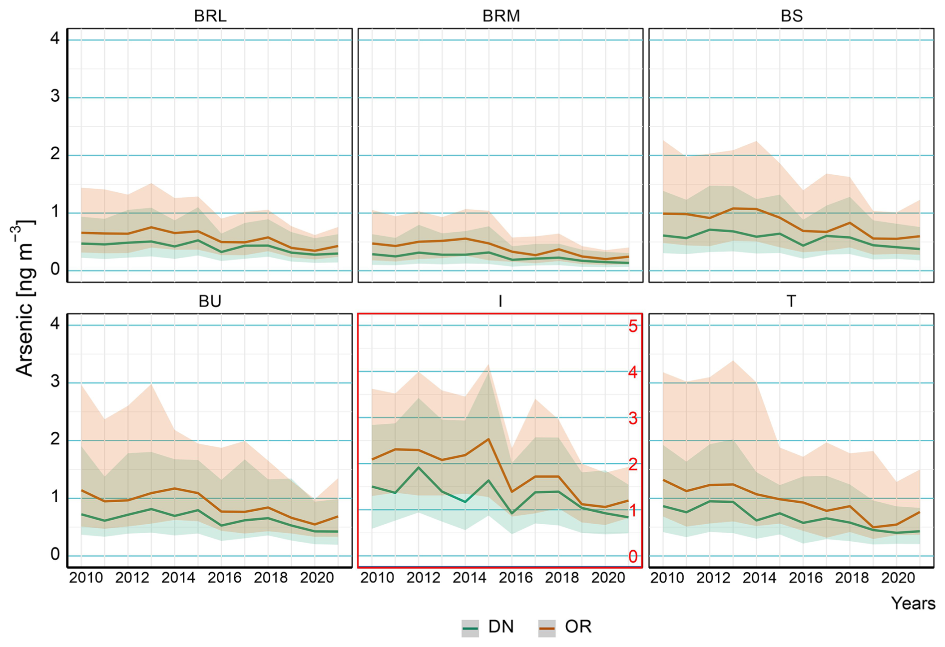
Figure 5 Arsenic concentration at background rural lowland (BRL) stations, background rural mountain (BRM) stations, background suburban (BS) stations, background urban (BU) stations, industrial (I) stations, and traffic (T) stations, 2010–2021. The green line represents the median concentration of dispersion-normalised data (DN), and the orange line represents the median concentration of the original data series (OR). The coloured area visualises the interquartile range (25th–75th percentile).

The cleanest monitoring environment was BRM, based on As_DN, with values ranging from 0.13 to 0.32 ng m⁻³ (Fig. 5).

Cadmium exhibited statistically significant declining trends across all station types (p < 0.001), with annual reduction rates ranging from 4.77 % (BRL) to 6.15 % (BS). The highest reduction rate at BS is likely connected to emission control measures, reflecting a combination of traffic emission reductions and decreased industrial activity in peri-urban zones. A pattern influenced by meteorology is evident during 2010–2014, when Cd_OR–Cd_DN ranged from 20 % to 52 % across all environments. However, from 2015, better dispersion conditions were observed (Cd_OR–Cd_DN: 8 %–46 %) at several stations (BRL, BRM, BS, BU, I), particularly in 2017. Cd_OR–Cd_DN convergence was likely a result not only of the stabilisation of meteorological conditions but also of the consistency of emission sources (Fig. 6).

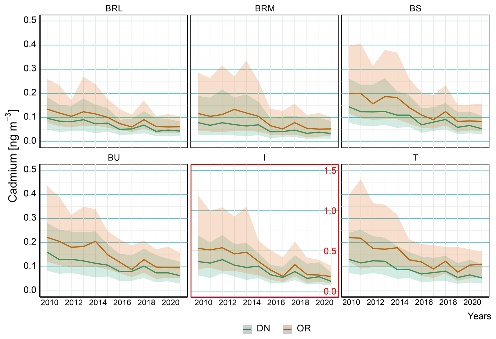
Figure 6 Cadmium concentration at background rural lowland (BRL) stations, background rural mountain (BRM) stations, background suburban (BS) stations, background urban (BU) stations, industrial (I) stations, and traffic (T) stations, 2010–2021. The green line represents the median concentration of dispersion normalising data (DN), and the orange line represents the median concentration of the original data series (OR). The coloured area visualises the interquartile range (25th–75th percentile).

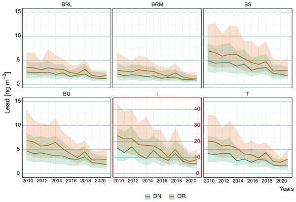
The evolution of Ni concentration was consistent with As, Cd, and Pb. Statistically significant declining trends were observed at all station types except the I station. Annual reduction rates ranging from 3.07 % (BS) to 5.02 % (T) showed no significant trends. The industrial sources likely suppress the regulatory measures more effectively than other HMs. Ni emissions were governed by sources with an operation regime less affected by seasonality, such as industrial processes and tyre and brake abrasion from traffic. The consistently high OR–DN divergence (20 %–50 %) indicates that atmospheric behaviour of Ni is sensitive to meteorological conditions, expressed in all environments (Fig. 7).

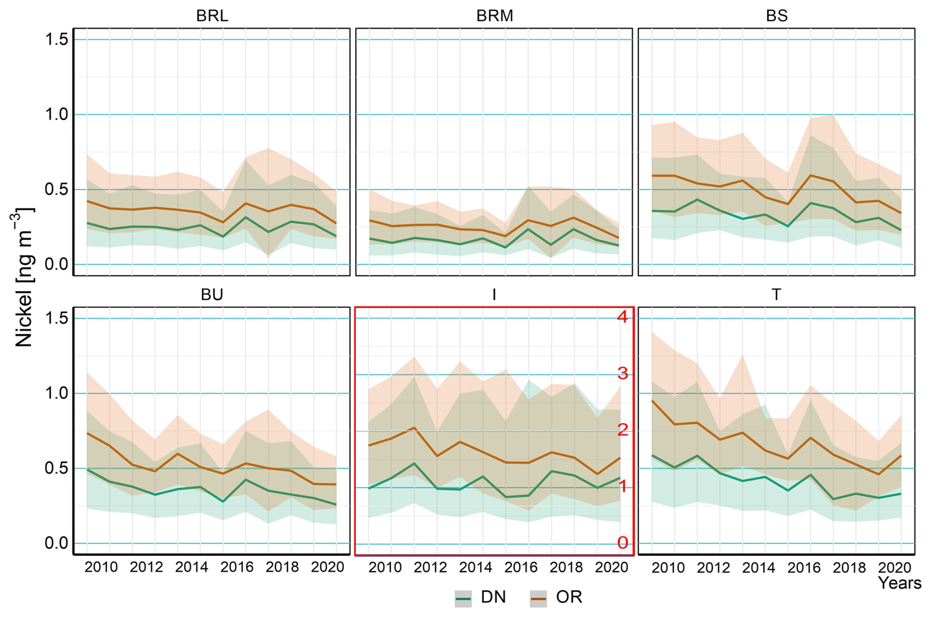
Figure 7 Nickel concentration at background rural lowland (BRL) stations, background rural mountain (BRM) stations, background suburban (BS) stations, background urban (BU) stations, industrial (I) stations, and traffic (T) stations, 2010–2021. The green line represents the median concentration of dispersion normalising data (DN), and the orange line represents the median concentration of the original data series (OR). The coloured area visualises the interquartile range (25th–75th percentile).

Lead showed the most pronounced concentration reductions across the monitoring network, with statistically significant declines at all station types (p < 0.001) and annual reduction rates ranging from 4.59 % (BRL) to 5.87 % (T). Pb concentrations at the I station type (6.07–16.69 ng m⁻³) were an order of magnitude higher than at BRM locations, which recorded the lowest concentrations (0.89–2.17 ng m⁻³). This steep decline in Pb_DN likely reflects the effectiveness of Pb phase-out policies in gasoline and industrial processes. Episodic peaks observed at the I station (2012, 2015, 2018) suggest that, despite overall declining trends, certain industrial processes continue to generate periodic increases in emissions. High meteorological sensitivity at T stations (8 %–50 % OR–DN divergence) combined with the highest reduction rate (5.87 %) indicates that, while traffic-related Pb emissions have declined substantially, street canyon effects continue to complicate the relationship between emissions and observed concentrations. The second-highest reduction rate in Pb_DN values was observed at BS station types (5.78 %) (Fig. 8).

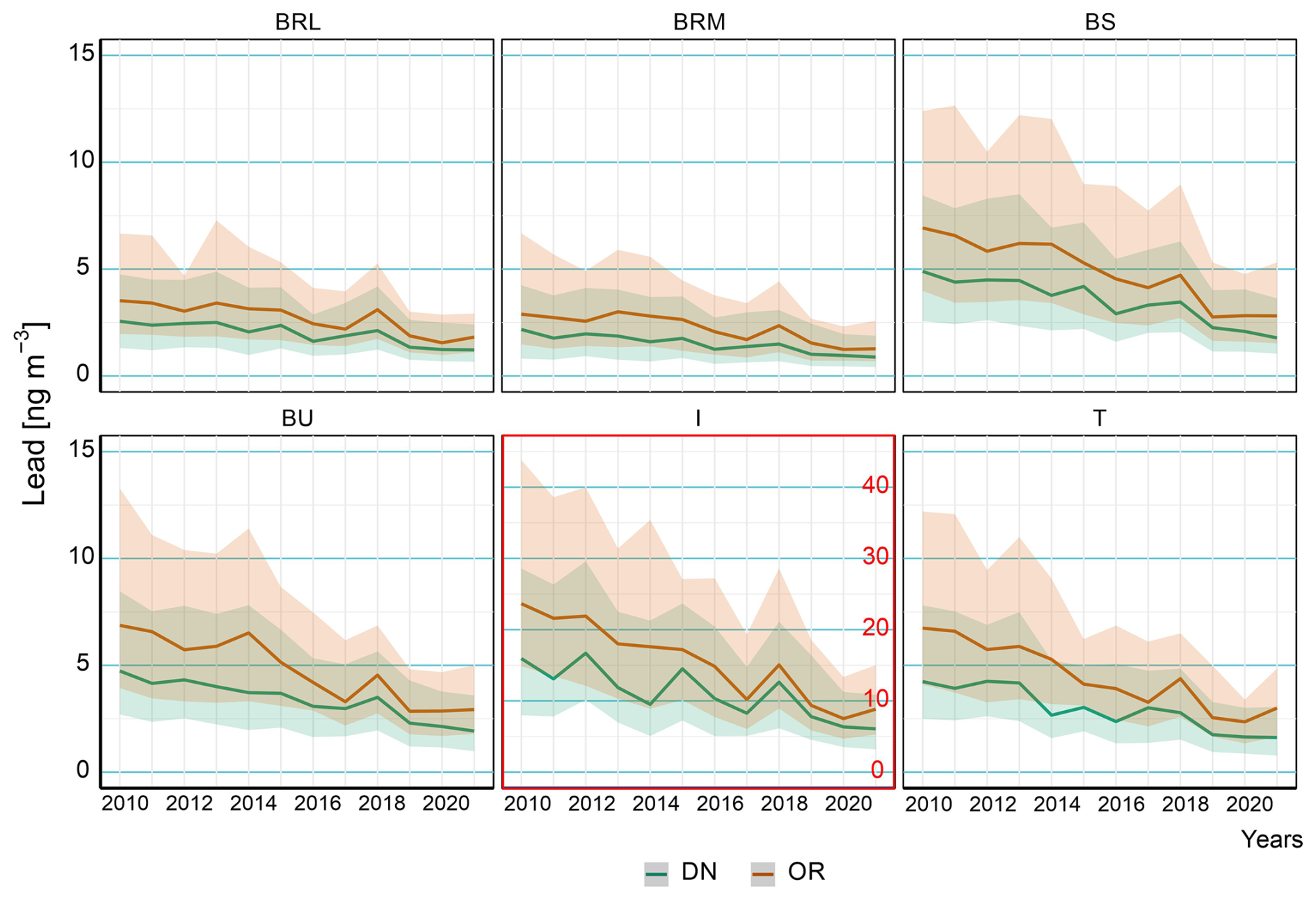
Figure 8 Lead concentration at background rural lowland (BRL) stations, background rural mountain (BRM) stations, background suburban (BS) stations, background urban (BU) stations, industrial (I) stations, and traffic (T) stations, 2010–2021. The green line represents the median concentration of dispersion-normalising data (DN), and the orange line represents the median concentration of the original data series (OR). The coloured area visualises the interquartile range (25th–75th percentile).

The dispersion conditions at the individual station are visualised in Figs. S3 and S4 according to the CHMI (2026b) method and Škáchová and Keder (2025).

5.7 Patterns across station types: BRL, BRM, BS, BU, I, T

BRL stations show consistent patterns for all HMs, characterised by a relatively narrow interquartile span, minimal temporal variability, and the lowest OR–DN divergence. This pattern was demonstrated by As_DN (0.28–0.51 ng m⁻³, 12 %–36 % divergence), Cd_DN (0.04–0.09 ng m⁻³, 13 %–35 % divergence), Ni_DN (0.13–0.27 ng m⁻³, 26 %–39 % divergence), and Pb_DN (1.37–2.88 ng m⁻³, 13 %–36 % divergence). Stable emission sources and minimal local anthropogenic influences could characterise the BRL environment. HM_DN concentrations (As, Cd, Ni, and Pb) demonstrate statistically significant declining trends (3.75 %, 4.77 %, 3.39 %, and 4.59 % annually, respectively; p < 0.001).

BRM stations recorded the lowest concentrations of HM (As_DN: 0.13–0.32 ng m⁻³; Cd_DN: 0.03–0.08 ng m⁻³; Ni_DN: 0.06–0.17 ng m⁻³; and Pb_DN: 0.89–2.17 ng m⁻³), confirming the least anthropogenically impacted monitoring locations. BRM stations are characterised by persistent OR–DN divergence (As: 20 %–50 %; Cd: 21 %–47 %; Ni: 31 %–49 %; Pb: 19 %–43 %; Table S11), indicating pronounced meteorological sensitivity. Long-range atmospheric transport and meteorological dispersion were likely to be the dominant factors controlling the HM concentrations in this clean environment. The BRM stations demonstrate the highest annual reduction rates for Cd_DN (5.93 %, p < 0.001), followed by reductions in As_DN (5.06 %, p <  0.001) and Pb_DN (4.75 %, p < 0.001) and Ni_DN (4.00 %, p < 0.001).

BS stations recorded the mean HM_DN concentration within the studied data series (As: 0.37–0.71 ng m⁻³; Cd: 0.05–0.14 ng m⁻³; Ni: 0.21–0.43 ng m⁻³; Pb: 1.77–4.89 ng m⁻³), reflecting the transitional nature between rural and urban environments. The highest annual reduction rates for Cd_DN (6.15 %, p < 0.001) and Pb_DN (5.78 %, p < 0.001) are likely a result of emission control measures. The OR–DN divergence at BS stations (As: 11 %–44 %; Cd: 11 %–40 %; Pb: 18 %–38 %; Table S11) could be influenced by both local and regional transport of pollutants and changes in meteorological conditions (except for Ni: 20 %–46 %).

BU stations observed concentration levels exceeding those at BRL and BS stations (As_DN: 0.42–0.81 ng m⁻³; Cd_DN: 0.06–0.16 ng m⁻³; Ni_DN: 0.21–0.49 ng m⁻³; Pb_DN: 1.92–4.74 ng m⁻³) with a broader interquartile span. The OR–DN divergence for individual HMs (As: 20 %–41 %; Cd: 8 %–44 %; Ni: 20 %–40 %; Pb: 9 %–42 %; Table S11) may be caused by fluctuating emission sources and the dynamics of meteorological conditions in the urban environment. The lowest annual reduction rates among all station types were observed for As_DN (3.46 %, p < 0.001); the remaining HMs showed decreases in Cd_DN (5.37 %), Pb_DN (5.72 %), and Ni_DN (3.66 %) (p < 0.001). Despite the gradual decline, the influence of local sources or unfavourable meteorological conditions occurred episodically in the BU environment (e.g. in 2014).

The industrial station consistently recorded the highest HM concentrations (As_DN: 0.83–1.91 ng m⁻³; Cd_DN: 0.12–0.36 ng m⁻³; Ni_DN: 0.83–1.42 ng m⁻³; Pb_DN: 6.07–16.69 ng m⁻³), confirming their proximity to major emission sources. Episodic emission events and the response to dispersion conditions were reflected in the OR–DN divergence (As: 7 %–47 %; Cd: 8 %–39 %; Ni: 20 %–47 %; Pb: 15 %–46 %; Table S11). The periodic influence of local emission sources was recorded, e.g. for Pb in 2012, 2015, and 2018. Despite the highest HM_DN concentrations, moderate annual reduction rates were observed (As_DN: 3.73 %; Cd_DN: 5.73 %; Pb_DN: 4.94 %; all p < 0.001). Ni_DN showed a slight, non-significant increase (0.74 %), suggesting that, although emission controls have been partially effective, industrial sources may still influence this type of station. Additionally, Ni_DN annual concentrations exceeded 1.00 ng m⁻³ in half of the study period, indicating the presence of Ni emission sources.

At the T station, concentration ranges were as follows: As_DN – 0.40–0.95 ng m⁻³; Cd_DN – 0.06–0.13 ng m⁻³; Ni_DN – 0.30–0.59 ng m⁻³; and Pb_DN – 1.62–4.26 ng m⁻³. High annual reduction rates were observed for all HMs – As_DN (4.50 %, p < 0.001), Cd_DN (5.20 %, p < 0.001), Ni_DN (5.02 %, p < 0.001), and Pb_DN (5.87 %, p < 0.001). The declining trend likely reflects a reduction in traffic-related emissions, thus indicating the effectiveness of policies targeting vehicular emissions, including fuel quality improvements and fleet modernisation. The OR–DN divergence range (As: 9 %–44 %; Cd: 20 %–52 %; Pb: 8 %–50 %; Ni: 27 %–50 %; Table S11) indicated the influence of both ground-level emissions and dispersion conditions associated with street canyon effects.

6 Discussion

The present study demonstrates that international and European legislative measures have had a positive effect on HM concentrations in ambient air in the Czech Republic while also highlighting the continued influence of industrial sources. The observed total annual declines in HM concentrations (1.7 %–8.1 % yr⁻¹) are substantially higher than the decline in total PM₁₀ concentrations across European background stations (1.8 % yr⁻¹) reported by Aas et al. (2024). This contrast supports the assumption that regulatory measures specifically targeting HM emissions have been more effective than general particulate matter mitigation strategies.

Comparable long-term trends were reported by Kyllönen et al. (2020), where HM concentrations at a subarctic background station in Finland were evaluated. However, their study identified lower levels of statistical significance for As (no significant trend), Cd and Ni (p < 0.05), and Pb (p < 0.001) during the overlapping period. In contrast, our results show statistically significant decreasing trends (p < 0.001) for most station types and metals, indicating that emission reduction measures may have had a stronger impact in Central Europe, where industrial density and historical emission burdens were considerably higher.

A notable feature in the time series is the elevated HM concentrations observed in 2018. This increase coincided with an exceptionally dry and warm spring–summer period that affected large parts of western, northern, and Central Europe (Bastos et al., 2020). The prolonged drought reduced wet deposition and enhanced atmospheric stability, leading to the accumulation of pollutants, including HMs in the atmosphere. Similar meteorologically driven increases in pollutant concentrations and deposition have been documented within the EMEP network (Travnikov et al., 2020). This finding supports the need for DN approaches to separate emission trends from meteorological variability.

The year 2018 serves as an example of how meteorological conditions can mask or amplify true emission signals in measured immission data. In the present study, the divergence between OR and DN concentrations reached up to 52 % across station types and individual metals, demonstrating a substantial impact of atmospheric dispersion conditions on measured concentrations, particularly during years with unfavourable dispersion conditions, notably in the cold season of 2010–2013. Another such example is the increase in As_OR and Cd_OR concentrations at a traffic station during 2020 and 2021, which could be incorrectly attributed to the impact of coronavirus-pandemic-related restrictions. However, our results suggest that these increases were more likely to be attributable to adverse meteorological dispersion conditions rather than changes in emission levels. Without DN, such meteorologically induced anomalies could be incorrectly interpreted as actual changes in emission levels.

The ventilation coefficient, which combines MLH and wind speed, proved to be an effective parameter in representing the dominant meteorological factors influencing pollutant dispersion. By applying DN, the underlying emission-driven trends become more identifiable, providing a more robust basis for assessing the effectiveness of legislative measures. This methodological approach is particularly valuable in datasets spanning multiple years, where interannual meteorological variability, as documented by Travnikov et al. (2020), who reported concentration changes of up to ±50 % attributable solely to meteorological variability, could otherwise obscure long-term trends.

The only location among all observed stations and HMs that exceeded the air pollution limit (specifically for As_OR) was the SKL station, classified as an urban background station. The annual air pollution limit for As_OR (6 ng m⁻³) was exceeded at this station in 2010, 2012, and 2013. The elevated As concentrations at this station are consistent with the influence of residential coal combustion, a well-documented source of As in urban environments, particularly during the heating season.

HM concentrations at urban stations in the Czech Republic are comparable to the mean values reported for two urban background stations in Germany during 2008–2010 (Dimitriou and Kassomenos, 2017). While As concentrations were higher at Czech urban stations, Cd and Pb concentrations at German urban stations were similar to those measured across Czech urban, industrial, and traffic sites. In contrast, Ni concentrations at German urban sites exceeded those observed at Czech industrial locations. In their study, traffic was identified as the dominant source of As, Cd, and Pb, whereas fuel oil combustion for residential heating was the primary source of Ni. These different source characteristics (traffic for As, Cd, and Pb vs. oil combustion for Ni) are consistent with the spatial patterns observed in our dataset, particularly the distinct behaviour of Ni at individual monitoring sites and the different trends of Ni at the industrial station.

According to the European Environment Agency EEA (2026), a continued overall decline in HM emissions has been observed across the EU, supporting the long-term effectiveness of legislative frameworks such as the CLRTAP Heavy Metals Protocol and EU air quality directives. Nevertheless, Germany and Poland – two countries bordering the Czech Republic – remain among the largest HM emitters in the EU. Notably, Poland showed one of the smallest reductions in Cd (−2.7 %) and Pb (−17.6 %) emissions between 2005 and 2023. Given the documented importance of transboundary transport in Central Europe (Travnikov et al., 2020), long-range transport may contribute to the measured concentrations in the Czech Republic, particularly at background and mountain sites. Additionally, Slovakia and Hungary have been reported among countries with relatively high Pb and Cd concentrations within the EMEP region, further supporting the regional dimension of HM pollution.

Our findings of declining Pb and Cd concentrations across the Czech Republic are consistent with the study of Hunová et al. (2023), in which depositional fluxes of these substances were examined and a decline in Pb and Cd deposition from 2012 to 2019 was observed.

The absence of a statistically significant trend in Ni concentrations at the industrial station is a notable exception within the dataset. This pattern may reflect the local specificity of Ni emission sources in the Ostrava region, where metallurgical processes are largely independent of seasonal cycles, in contrast to combustion-related sources that drive trends in other HMs (Font et al., 2022).

7 Conclusions

The long-term trend of HMs at different station types in the Czech Republic was evaluated and showed a decreasing trend at the highest statistical significance level (p < 0.001) during the period 2010–2021. The results confirm the positive impact of regulatory measures implemented after 2008. Given the Czech Republic's central location and its exposure to regional emission patterns, the findings may also be relevant to the wider Central European context as outlined in objective 1 in the Introduction.

A total of 16 stations with daily measurements over a 12-year period were studied, and the groups were evaluated according to their classification and spatial locations. The representativeness of the group was confirmed by the statistical significance of HM concentrations at individual stations (p < 0.001). A total of 9 % of cases (6 results from 64) did not confirm the decreasing trend observed at the rest of the stations, which was likely due to a specific pollution source at the location. The correlation analyses showed the spatial connection between the stations, especially for Cd_DN and Pb_DN. Low correlations were found for Ni_DN across all stations (R_s = 0.22–0.52). Three features characterise mountain sites: low HM concentrations, weak inter-station correlations (R_s < 0.7), and a relatively stable OR–DN difference (19 %–51 %). This indicates a significant influence of dispersion conditions on HM concentrations. Generally, it was confirmed that grouping stations by classification yields representative results for station and environmental types. However, the specificity of pollution sources must be taken into account, and so more than one station is recommended for calculating the representative group (see point 2 in the set objectives in the Introduction).

The DN data evolution clearly demonstrated the results of regulatory measures. Specific meteorological conditions were observed across the range of station environments, from mountain locations to street canyons. The OR–DN ratio confirms the potential of meteorological conditions to mask the real emission level. Our results confirm that, when evaluating HM emission regulations, the use of DN can provide clearer results. Although, in this study, the VC was obtained from the Aladin model, which is not available to the broad user community, the variables used to calculate the ventilation coefficient are accessible via sources such as the Hysplit model (e.g. Rolph et al., 2017; Stein et al., 2015) or ERA5 (Copernicus Climate Change Service, 2023). The user community can apply the DN method without significant limitations.