Photocatalytic chloride-to-chlorine conversion by ionic iron in aqueous aerosols: a combined experimental, quantum chemical, and chemical equilibrium model study

Prior aerosol chamber experiments show that the ligand-to-metal charge transfer absorption in iron(III) chlorides can lead to the production of chlorine (Cl₂/Cl). Based on this mechanism, the photocatalytic oxidation of chloride (Cl⁻) in mineral dust–sea spray aerosols was recently shown to be the largest source of chlorine over the North Atlantic. However, there has not been a detailed analysis of the mechanism that includes the aqueous formation equilibria and the absorption spectra of the iron chlorides nor has there been an analysis of which iron chloride is the main chromophore. Here we present the results of experiments measuring the photolysis of FeCl₃ ⋅ 6H₂O in specific wavelength bands, an analysis of the absorption spectra of FeCl${}_n^{\mathrm{3}-n}$ (n=1 … 4) made using density functional theory, and the results of an aqueous-phase model that predicts the abundance of the iron chlorides with changes in pH and iron concentrations. Transition state analysis is used to determine the energy thresholds of the dissociations of the species. Based on a speciation model with conditions extending from dilute water droplets and acidic seawater droplets to brine and salty crust, as well as the absorption rates and dissociation thresholds, we find that FeCl${}_{\mathrm{2}}^{+}$ is the most important species for chlorine production for a wide range of conditions. The mechanism was found to be active in the range of 400 to 530 nm, with a maximum around 440 nm. We conclude that iron chlorides will form in atmospheric aerosols from the combination of iron(III) cations with chloride and that they will be activated by sunlight, generating chlorine (Cl₂/Cl) from chloride (Cl⁻) in a process that is catalytic in both chlorine and iron.

1 Introduction

Common components of atmospheric mineral dust, including TiO₂ and Fe₂O₃, are photocatalytically active (Ponczek and George, 2018), and yet evidence of this playing a meaningful role in the atmospheric radical budget has been elusive (Abou-Ghanem et al., 2020; Chen et al., 2012). Recently, a large new source of chlorine atoms was discovered as a result of the combination of Sahara dust with sea spray aerosol over the North Atlantic (van Herpen et al., 2023). The mechanism is triggered when Sahara dust mixes with sea spray aerosol in the marine boundary layer. Iron from the Sahara dust is released and forms iron chlorides with chloride from the sea spray. Iron chlorides can absorb sunlight, releasing a chlorine atom. The chlorine is emitted from the aerosol as molecular chlorine (Cl₂), which is then photolyzed by sunlight to yield atomic Cl in the gas phase (Wittmer et al., 2015, 2016; Wittmer and Zetzsch, 2017). The chlorine produced by mineral dust–sea spray aerosols is estimated to produce 41 % of the chlorine over the Atlantic, thus impacting methane directly (Cl + CH₄) and indirectly (reduction in [O₃] from Cl + O₃ reduces OH source). (Oeste, 2009) proposed a method for intentionally increasing the production of chlorine using iron salt aerosol to achieve atmospheric methane removal (AMR) (Oeste, 2009; Meyer-Oeste, 2014). The use of chlorine from any source as a climate intervention was recently evaluated by Li et al. (2023).

Traditionally, the tropospheric chlorine cycle (Saiz-Lopez and von Glasow, 2012; Simpson et al., 2015) begins with the formation of sea spray aerosol (Nielsen and Bilde, 2020), which is known to be comprised of particles with high acidity (Angle et al., 2021). Acids such as HNO₃ and H₂SO₄ deposit, forcing HCl into the gas phase, which can react with OH to produce chlorine atoms, HCl + OH → Cl + H₂O (Young et al., 2014). Cl reacts with ozone, impacting the formation of hydroxyl radicals, and it reacts with methane and other hydrocarbons, reforming HCl (Chang and Allen, 2006; Knipping and Dabdub, 2003; Badia et al., 2019).

Chlorine production is poorly constrained, and as a result, Cl is estimated to remove between 0.8 % and 3.3 % of tropospheric methane, depending on the model (Allan et al., 2007; Hossaini et al., 2016; Sherwen et al., 2016; Gromov et al., 2018; Li et al., 2022). Multiple lines of evidence show that chlorine concentrations in the troposphere exceed what can be explained with existing mechanisms. These include (1) ¹³C depletion in CO in air samples from Barbados (Mak et al., 2003), which is a signature of methane oxidation by chlorine; (2) anomalies in the CO : ethane ratio seen at Cabo Verde (Read et al., 2009); and (3) observations of elevations in the concentration of HOCl above what can be explained with standard chemistry (Lawler et al., 2011). (4) Finally, a comprehensive simulation of tropospheric chlorine using the Goddard Earth Observing System with Chemistry (GEOS-Chem) global 3-D model of oxidant–aerosol–halogen atmospheric chemistry could not explain the elevated Cl₂ mixing ratios measured in the boundary layer in the WINTER aircraft campaign (Wang et al., 2019).

Additional chlorine production impacts our understanding of the methane budget because the abundance of ¹³C in atmospheric methane is used to constrain emission sources and because Cl + CH₄ has a large kinetic isotope effect, while the main atmospheric methane sink reaction OH + CH₄ does not. The reaction of CH₄ with Cl has a carbon kinetic isotope effect (KIE) of ^13CKIE_Cl=1.066 (±0.002) at 297 K, which is around 17 times more fractionating than methane oxidation with OH radicals (Saueressig et al., 2001; Cantrell et al., 1990; Saueressig et al., 1995). The discovery of a new chlorine source means that methane sources must be more depleted than had been recognized, leading to the conclusion that previous methane emissions budgets, which did not include the new chlorine source, likely underestimate biogenic methane (e.g., wetlands and agriculture) and overestimate the fossil fuel source (van Herpen et al., 2023). To understand the methane budget, it is imperative to fully characterize the chlorine production mechanism and to see how it will vary with chemical conditions such as pH, chloride concentration, and the concentrations of possibly interfering ions.

Historically, iron(III) chloride has been believed to form four complexes, namely FeCl²⁺, FeCl${}_{\mathrm{2}}^{+}$, FeCl₃, and FeCl${}_{\mathrm{4}}^{-}$ (Gamlen and Jordan, 1953). Uchikoshi et al. (2022) presented a model of iron(III) chloride species, which shows the most plausible species to be FeCl${}_{\mathrm{2}}^{+}$, FeCl₃, FeCl${}_{\mathrm{4}}^{-}$, and FeCl${}_{\mathrm{6}}^{\mathrm{3}-}$. With the use of a theoretical mathematical decomposition model called the multivariate curve resolution–alternative least squares (MCRALSs) and a five-complex model, they determined that the combination of Cl coordination numbers is n=0, 2, 3, 4, and 6. That study indicates that FeCl²⁺ will not be formed, and the highest chlorinated complex, forming at the highest chloride concentrations, will be FeCl${}_{\mathrm{6}}^{\mathrm{3}-}$. The research by Uchikoshi et al. (2022) shows FeCl${}_{\mathrm{2}}^{+}$, FeCl₃, and FeCl${}_{\mathrm{4}}^{-}$ forming at a lower chloride concentration than previously expected. However, FeCl${}_{\mathrm{6}}^{\mathrm{3}-}$ has not been implemented in this study.

In this study, we present a detailed description of the photocatalytic oxidation of chloride to chlorine, based on four iron(III) chloride complexes, namely FeCl²⁺, FeCl${}_{\mathrm{2}}^{+}$, FeCl₃, and FeCl${}_{\mathrm{4}}^{-}$. A combination of modeling, quantum chemical calculations, and laboratory experiments explains the formation constants of the iron chlorides under changing conditions of pH and chloride concentration, their absorption rates under tropospheric sunlight, the quantum yield of absorption resulting from the energy threshold for photodissociation to yield a Cl radical, and the production of Cl₂ from irradiation of FeCl₃⋅ 6H₂O.

1.1 The Fe(III)Cl_n³⁻ⁿ system

Various Fe(III) complexes form in marine boundary layer aerosol, where the speciation depends on pH, salt composition, chloride concentration, water activity, and ionic strength. The Pourbaix diagram of aqueous iron shows that dissolved iron will be in the form of free Fe(III) and not Fe(OH)₃, Fe(II), or Fe(OH)₂, given acidic and oxidizing conditions (pH < 3.6 and E_H>0.72 V) (Harnung and Johnson, 2012). Given the presence of chloride and Fe(III), the iron(III) chlorides will form.

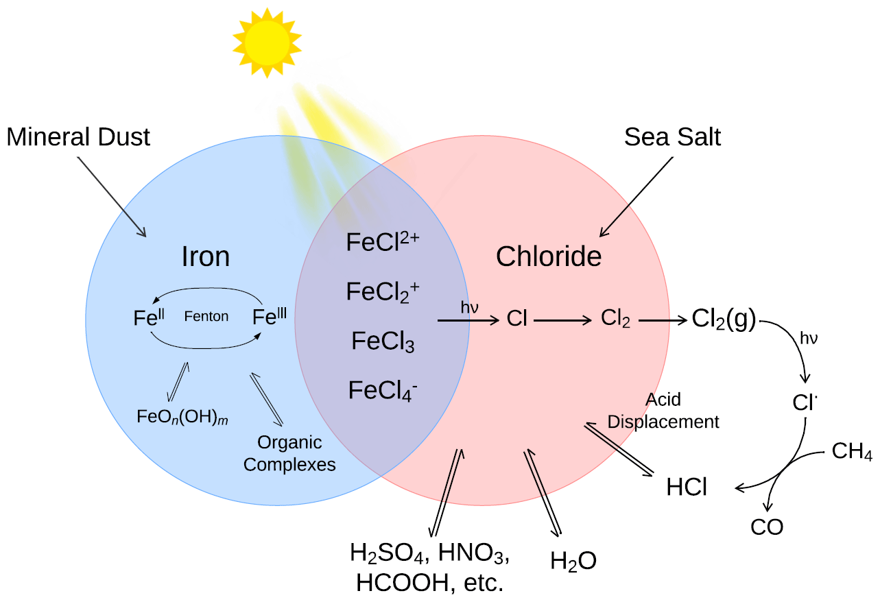
Figure 1 The primary sources and sinks for iron(II) and iron(III) ions and chloride in the atmospheric aerosols and their influence on the formation of iron(III) chlorides in a low pH environment.

The central Fe(III)Cl_n³⁻ⁿ reactions that occur in an aerosol or the marine boundary layer are shown in Reaction (R1) for n=0 … 3 (Lindén et al., 1993).

$$\begin{array}{}\text{(R1)}& {\mathrm{FeCl}}_n^{\mathrm{3}-n}+{\mathrm{Cl}}^{-}\rightleftharpoons {\mathrm{FeCl}}_{n+\mathrm{1}}^{\mathrm{2}-n}\end{array}$$

Iron(III) chloride formation may be inhibited by the presence of other ions, such as sulfate or fluoride, or by organic compounds, such as oxalates that bind with Fe(III).

The photolysis of the iron(III) chlorides is shown in a general form in Reaction (R2) for n≥1. In this ligand to metal electron transfer absorption, Fe(III) is reduced to Fe(II), and chloride is oxidized, yielding a chlorine atom (Lindén et al., 1993; Nadtochenko and Kiwi, 1998).

$$\begin{array}{}\text{(R2)}& {\mathrm{FeCl}}_n^{\mathrm{3}-n}+h\mathit{\nu }\to {\mathrm{FeCl}}_{n-\mathrm{1}}^{\mathrm{3}-n}+\mathrm{Cl}\cdot \end{array}$$

For example, for n=1, Reaction (R2) has a quantum yield of 0.5 ± 0.1 at a wavelength of 347 nm. At higher pH, the formation of iron(III) chloride complexes competes with iron hydroxide complexes (also depending on [Cl⁻]), as seen in Reactions (R3) and (R4).

$$\begin{array}{}\text{(R3)}& {\mathrm{Fe}}^{\mathrm{3}+}+{\mathrm{OH}}^{-}\rightleftharpoons {\mathrm{FeOH}}^{\mathrm{2}+}\end{array}$$

$$\begin{array}{}\text{(R4)}& {\mathrm{FeOH}}^{\mathrm{2}+}+{\mathrm{OH}}^{-}\rightleftharpoons \mathrm{Fe}(\mathrm{OH}{)}_{\mathrm{2}}^{+}\end{array}$$

Iron(III) hydroxide complexes can be photolyzed, similar to iron(III) chlorides; however, only some of the iron is photoreduced. Reaction (R5) produces OH radicals with a quantum yield of 0.21 ± 0.04 at a wavelength of 347 nm (Nadtochenko and Kiwi, 1998), whereas Reaction (R6) shows that the photolysis of Fe(OH)${}_{\mathrm{2}}^{+}$ does not grant a reduction in the iron (Loures et al., 2013; Korte et al., 2011).

$$\begin{array}{}\text{(R5)}& \mathrm{Fe}(\mathrm{OH}{)}^{\mathrm{2}+}+h\mathit{\nu }\to {\mathrm{Fe}}^{\mathrm{2}+}+{\mathrm{OH}}^{\cdot }\end{array}$$

$$\begin{array}{}\text{(R6)}& \mathrm{Fe}(\mathrm{OH}{)}_{\mathrm{2}}^{+}+h\mathit{\nu }\to {\mathrm{FeOH}}^{\mathrm{2}+}+{\mathrm{OH}}^{-}\end{array}$$

In the aerosol process, the Fe(II) product is oxidized back to Fe(III) by one half of the Fenton process. In one example, for marine mineral aerosol, Zhu et al. (1993) found the oxidation rate to be 0.19 min⁻¹. The Fenton process describes how Fe(II) and Fe(III) act as a catalyst pair, breaking down hydrogen peroxide and generating radicals (Fenton, 1894). The Fenton reactions are shown in Reactions (R7) to (R9). Hydroxyl may react or escape to the gas phase.

$$\begin{array}{}\text{(R7)}& {\mathrm{Fe}}^{\mathrm{2}+}+{\mathrm{H}}_{\mathrm{2}}{\mathrm{O}}_{\mathrm{2}}\to {\mathrm{Fe}}^{\mathrm{3}+}+\mathrm{OH}\cdot +{\mathrm{OH}}^{-}\end{array}$$

$$\begin{array}{}\text{(R8)}& {\mathrm{Fe}}^{\mathrm{3}+}+{\mathrm{H}}_{\mathrm{2}}{\mathrm{O}}_{\mathrm{2}}\to {\mathrm{Fe}}^{\mathrm{2}+}+{\mathrm{HO}}_{\mathrm{2}}\cdot +{\mathrm{H}}^{+}\end{array}$$

$$\begin{array}{}\text{(R9)}& \mathrm{Net}:\mathrm{2}{\mathrm{H}}_{\mathrm{2}}{\mathrm{O}}_{\mathrm{2}}\to \mathrm{OH}\cdot +{\mathrm{HO}}_{\mathrm{2}}\cdot +{\mathrm{H}}_{\mathrm{2}}\mathrm{O}\end{array}$$

Wittmer and Zetzsch (2017) proposed that the production of OH will enhance Cl₂ production due to the production of a chlorine radical, as shown in Reactions (R10) to (R12). This route could be enhanced in chloride-rich environments. Several sources of OH are known, including photocatalytic minerals (Chen et al., 2012) and Fenton degradation of H₂O₂ in Reaction (R7).

$$\begin{array}{}\text{(R10)}& {\mathrm{OH}}^{\cdot }+{\mathrm{Cl}}^{-}\to {\mathrm{ClOH}}^{\cdot -}\end{array}$$

$$\begin{array}{}\text{(R11)}& {\mathrm{ClOH}}^{\cdot -}+{\mathrm{H}}^{+}\to {\mathrm{ClOH}}_{\mathrm{2}}^{\cdot }\end{array}$$

$$\begin{array}{}\text{(R12)}& {\mathrm{ClOH}}_{\mathrm{2}}^{\cdot }\to \mathrm{Cl}\cdot +{\mathrm{H}}_{\mathrm{2}}\mathrm{O}\end{array}$$

Reactions (R10) to (R12) take place in the aqueous phase. For the chloride produced in Reaction (R2) and the chlorine radical in Reaction (R12) to impact gas-phase chemistry, it must escape the particle. In the following, Reactions (R13) and (R14) lead to the production of Cl₂(aq) in Reaction (R15).

$$\begin{array}{}\text{(R13)}& {\mathrm{Cl}}^{-}+\mathrm{Cl}\cdot \rightleftharpoons {\mathrm{Cl}}_{\mathrm{2}}^{-}\end{array}$$

$$\begin{array}{}\text{(R14)}& \mathrm{2}{\mathrm{Cl}}_{\mathrm{2}}^{-}\rightleftharpoons {\mathrm{Cl}}_{\mathrm{2}}+\mathrm{2}{\mathrm{Cl}}^{-}\end{array}$$

$$\begin{array}{}\text{(R15)}& {\mathrm{Cl}}_{\mathrm{2}}^{-}+\mathrm{Cl}\cdot \rightleftharpoons {\mathrm{Cl}}_{\mathrm{2}}+{\mathrm{Cl}}^{-}\end{array}$$

Chlorine atoms may be lost before escaping as molecular chlorine in the gas phase. Possible mechanisms include the failure of the chlorine atom produced by photolysis to escape the solvent cage or diffuse back into contact, leading to the reformation of the iron chloride and the reaction of chlorine atoms with condensed-phase hydrocarbons forming HCl/Cl⁻.

Once in the gas phase, molecular chlorine is activated by light, as shown in Reaction (R16). Cl₂(g) absorbs in a band centered at 330 nm (Maric et al., 1993).

$$\begin{array}{}\text{(R16)}& {\mathrm{Cl}}_{\mathrm{2}}\left(g\right)+h\mathit{\nu }\to \mathrm{2}\mathrm{Cl}\cdot \left(g\right)\end{array}$$

Table 1 Species and initial concentrations listed for each aqueous equilibrium model (AEM) scenario. Two different iron concentrations are used for the iron seawater concentration, marked S, and iron aerosol concentration, marked A.

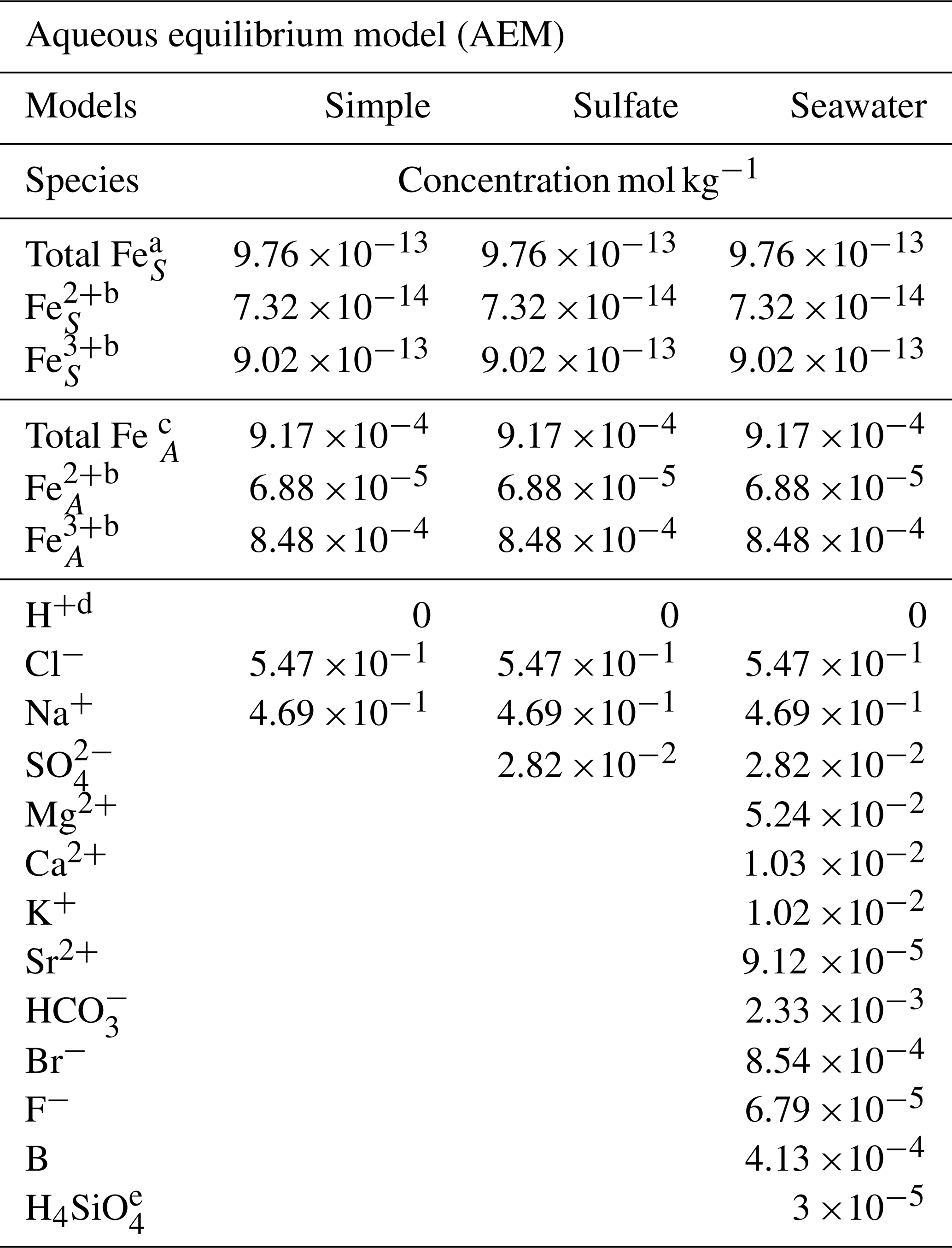
^a The mean value of the total iron concentration in seawater was obtained from Achterberg et al. (2001). ^b The ratio of Fe²⁺ and Fe³⁺ is 7.5 % and 92.5 %, respectively, and was obtained from Zhu et al. (1993). ^c The total iron concentration in aerosols was obtained from Hsu et al. (2010). ^d The required species for the AEM. ^e The value was obtained from Harnung and Johnson (2012). The concentrations for unmarked species are found in Stumm and Morgan (2012).

2 Methods

This section will include details of the study divided into the following three main parts: aqueous equilibrium model (AEM) (modeling the concentrations of FeCl${}_n^{\mathrm{3}-n}$ species), ab initio calculations (estimating absorption rates), and laboratory experiments (proving the formation of chloride from photolysis of FeCl${}_n^{\mathrm{3}-n}$ species).

2.1 Aqueous equilibrium model methods

Visual MINTEQ is a chemical equilibrium model that calculates the equilibrium speciation for the input species and predicts their concentration (Gustafsson, 2014). The program has been used to evaluate species with direct or indirect effects on iron(III)-induced chloride production.

Three AEM scenarios are shown in Table 1 and called simple, sulfate, and seawater. The species FeCl²⁺, FeCl${}_{\mathrm{2}}^{+}$, and FeCl₃ were manually added to the database, as shown in the Appendix Table A1 (Tagirov et al., 2000); however, FeCl${}_{\mathrm{4}}^{-}$ could not be added because the thermodynamic data are not available. Two different iron concentrations correlating to seawater and aerosol concentrations are used in all models, where the ratio between Fe²⁺ and Fe³⁺ is estimated to be 7.5 % to 92.5 % (Achterberg et al., 2001; Hsu et al., 2010; Zhu et al., 1993). The simple model shows the relation between iron chloride species, the sulfate model evaluates the potential effect of SO${}_{\mathrm{4}}^{\mathrm{2}-}$ on iron chlorides, and the seawater model includes all major ions found in seawater (Harnung and Johnson, 2012; Stumm and Morgan, 2012). The results from each of the three models are shown as species concentrations, and iron species are shown as a fraction of total iron as a function of pH in Sect. 3.1.

2.2 Ab initio calculations

Figure 2 describes the computational method, initialized by the generation of the molecules in GaussView, followed by geometry optimizations in vacuum (Frisch et al., 2016). The density functional theory method CAM-B3LYP/6-311++G(d,p) was used for all calculations (Yanai et al., 2004; Francl et al., 1982; McLean and Chandler, 1980; Spitznagel et al., 1987). Solvents were modeled using the PCM model (Tomasi et al., 1999). The relative permittivity, ϵ_r, for the solvents is in Table 2. See Appendix A2 for the geometries of the iron(III) chlorides.

Figure 2 Overview of the computational strategy, highlighting the key components of the relative permittivity (ϵ_r), transition state (TS), and time-dependent density functional theory (TD-DFT).

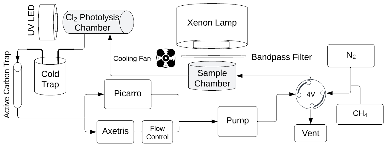
Figure 3 Overview of the system used in the laboratory experiments. The sample is located in the sample chamber. The volume S of the sample and Cl₂ photolysis chambers are 0.36 and 0.45 L, respectively. The four-port valve, 4V, changes the system between flow and loop mode.

Table 2 The set of relative permittivities (relative permittivity, ϵ_r) used to represent various solvents with the PCM model.

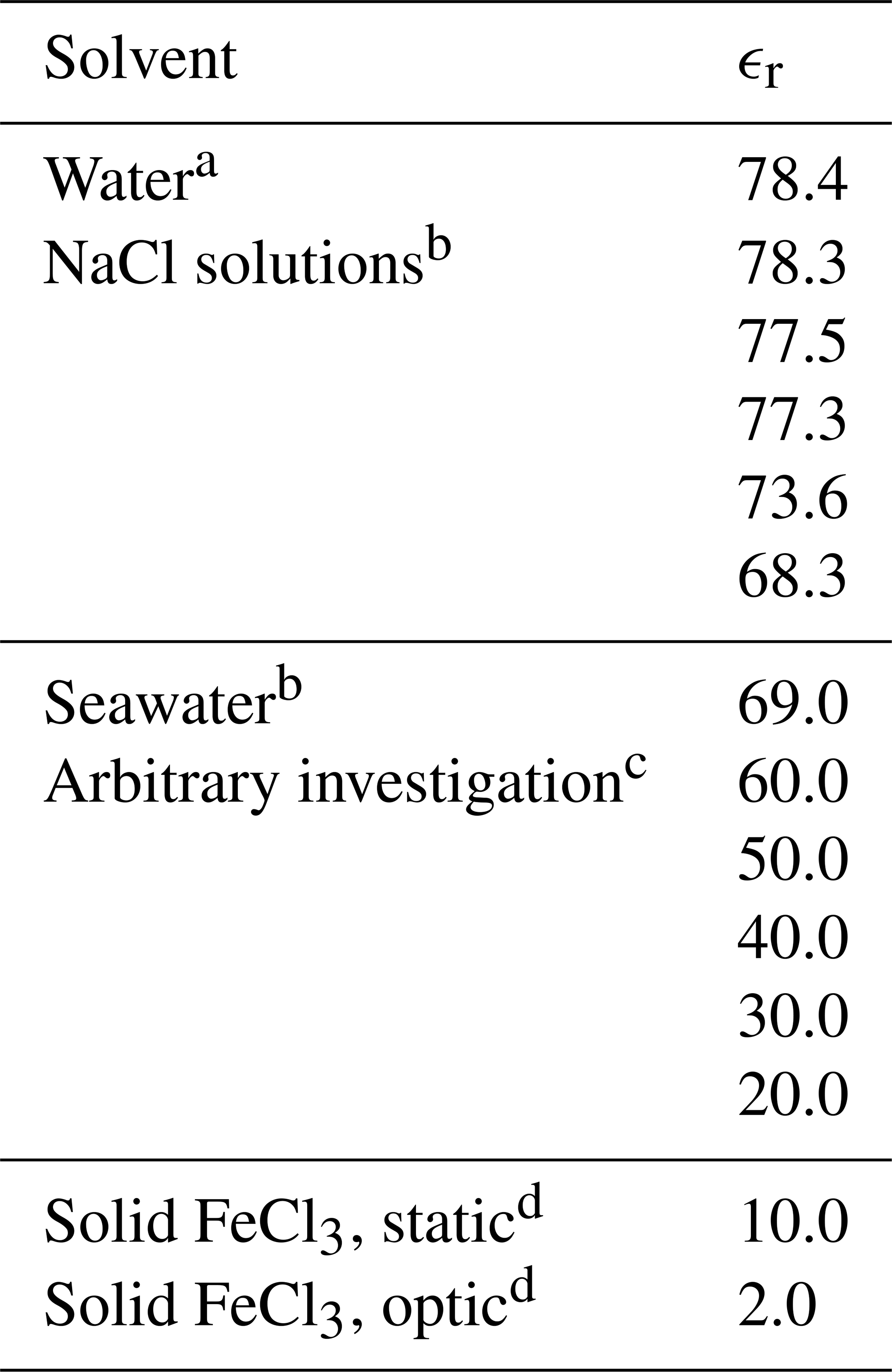
^a Value obtained from GaussView (Frisch et al., 2016). ^b Values obtained from Midi et al. (2014). ^c Arbitrary values were used for FeCl₃ only. ^d Estimations.

A transition state scan was made to evaluate the bond dissociation energy. In a few cases (mainly FeCl${}_{\mathrm{4}}^{-}$) in some solvents, the TS optimizations did not converge. TD-DFT calculations were used to explore the excitation energies of the molecules. Photolysis rates j_A were calculated using Eq. (1).

$$\begin{array}{}\text{(1)}& j_{\mathrm{A}}=\underset{{\mathit{\lambda }}_{\mathrm{1}}}{\overset{{\mathit{\lambda }}_{\mathrm{2}}}{\int }}{\mathit{\varphi }}_{\mathrm{A}}\left({\mathit{\lambda }}_{,}T\right)\cdot {\mathit{\sigma }}_{\mathrm{A}}\left({\mathit{\lambda }}_{,}T\right)\cdot I\left(\mathit{\lambda }\right)\mathrm{d}\mathit{\lambda },\end{array}$$

where the variables represent the molecular absorption cross section, σ_A (cm²); spectral actinic flux, I (n_hν cm⁻² s⁻¹ nm⁻¹); and quantum yield, ϕ_A (set to 1) (Seinfeld and Pandis, 2008). The absorption cross section was evaluated computationally, and the spectral actinic flux was determined using the Tropospheric Ultraviolet and Visible (TUV) radiation model for conditions corresponding to the marine boundary layer in the Atlantic, west of Cabo Verde (18.97° N, 39.12° W; 18 July 2022, 12:00) (Madronich et al., 2002).

2.3 Experimental method

The experimental system is shown in Fig. 3. Gases are introduced with a four-port valve (4V), which was used to select a flow-through or loop pattern. The average flow was measured to be 125 mL min⁻¹. A sample of FeCl₃⋅ 6H₂O was placed in the sample chamber (volume 0.36 L) illuminated by a xenon lamp. For wavelength-controlled experiments, a bandpass filter is placed on top of the sample chamber. The Cl₂ photolysis chamber is a photolysis chamber with a volume of 0.45 L and a high-power UV LED light source that ensures that the chlorine emitted by the sample in the sample chamber is photolyzed. The cold trap and active carbon trap ensure that organic molecules and carbon dioxide are captured, which protects the instruments and removes possible interference. The airflow is divided for analysis by the Picarro G2201-i Isotopic Analyzer for ${\mathrm{CO}}_{\mathrm{2}}/{\mathrm{CH}}_{\mathrm{4}}$ and the Axetris LGD Compact-A CH₄, which measure CH₄, δ¹³CH₄, CO₂, and H₂O. The flow controller is set to 125 mL min⁻¹, and the pump ensures flow through the system.

At the beginning of every experiment, the active carbon trap and cold trap are flushed, and a new sample of 20 mg FeCl₃⋅6H₂O in a 10 mL beaker is placed in a cleaned sample chamber. Methane is introduced to achieve a nominal mole fraction of 95 ppm, and the system is switched to loop mode. The concentrations of methane and carbon dioxide are monitored, and a leak test of the system is performed after the concentrations have stabilized. System stability is monitored for 10 min,, the xenon lamp is turned on for 15 min, and finally, an additional 10 min of measurement are taken to verify the system stability. The duration of an experiment is from 1.5 to 2.5 h. Three repetitions were made for each bandpass filter. The experimental procedure is described in greater detail in Appendix Fig. A1.

Two light sources were used, namely a xenon lamp from Eimac (see Fig. 4) and a UV LED (Luminus SST-10-UV Surface Mount LED lamp) (see Appendix Fig. A2). The spectrum of the xenon lamp is shown with a dashed line in Fig. 4; the light that enters the sample chamber is illustrated with a solid line. The legend name refers to the center wavelength of the bandpass filter in nanometers. The system and measurements of the sample chamber, bandpass filters, and the xenon lamp are illustrated in Appendix Fig. A3.

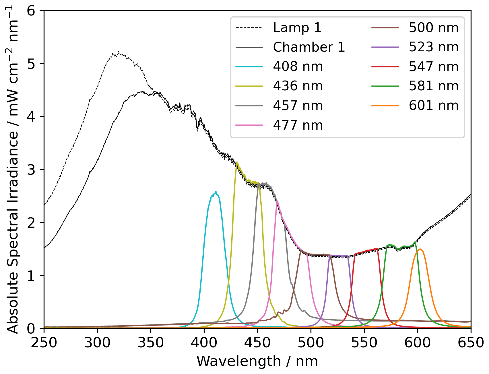
Figure 4 The measured absolute spectral irradiance of the xenon lamp before and after the sample chamber, including bandpass filters. Data are recorded with an Ocean Optics spectrometer.

3 Results

The results are presented in three sections, namely aqueous equilibrium modeling, ab initio calculations, and laboratory experiments.

Figure 5 Three AEM scenarios with a seawater iron concentration of 9.76 $\times {\mathrm{10}}^{-\mathrm{13}}$ mol kg⁻¹ (Fe_S) at 20 °C. All species below 5 % are shown in Appendix B2. See Appendix B3 and B4 for AEM scenarios with increased sulfate and iron concentrations, e.g., Fe(OH)₃.

3.1 Aqueous equilibrium modeling

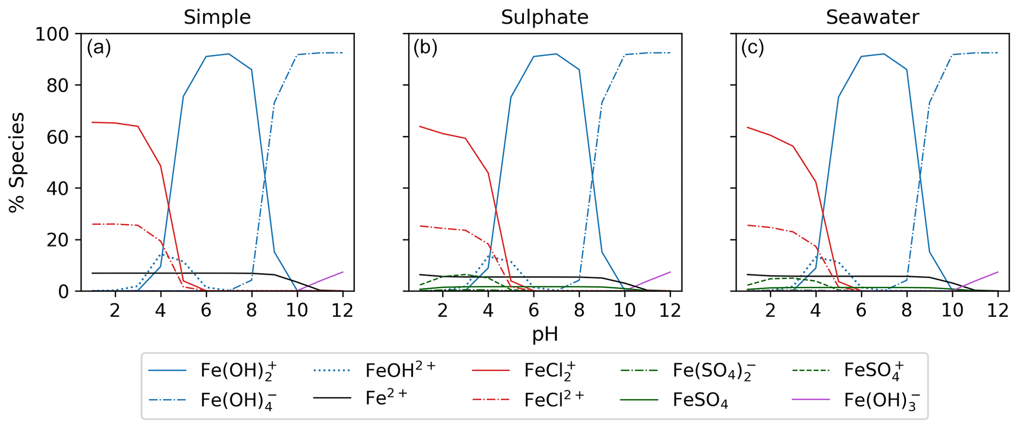
Figure 5 displays the iron speciation from the three AEM scenarios as a function of pH for the seawater iron concentration of 9.76 $\times {\mathrm{10}}^{-\mathrm{13}}$ mol kg⁻¹. Iron(III) chlorides are stable at pH values less than 4. Above this, the dominant species are iron hydroxides. This trend is consistent for all models in Fig. 5. According to the AEM scenarios, the two dominant iron(III) chloride species are FeCl²⁺ and FeCl${}_{\mathrm{2}}^{+}$, both observed in a low pH environment. The sulfate model (Fig. 5b), shows a slight decrease in the iron(III) chloride concentrations in the same pH range as the iron sulfates. However, increasing the sulfate concentration by a factor of 10 shows that sulfate is able to block the availability of some iron to form iron chlorides (see Appendix Fig. B3). In this scenario, sulfate changes the iron(III) chloride concentration by up to 40 % compared to the simple model. The seawater model (Fig. 5c) does not show any major changes compared to the sulfate model. Moreover, this is consistent for the scenarios with increased sulfate and iron concentration shown in Appendix Figs. B3 and B4. According to this study, sulfates are the main seawater anion that compete for iron(III) with chloride. Increasing the sulfate and iron concentration has a small impact on the speciation of iron fluorides, and as seen in the Appendix, all models are shown. The fraction of iron fluorides is below 5 %, and they will not be discussed further.

The temperature dependence of FeCl²⁺ and FeCl${}_{\mathrm{2}}^{+}$ was modeled with the seawater scenario of the AEM illustrated in Fig. 6 from 0 to 100 °C. The fraction of FeCl²⁺ increases with increasing temperature, and the opposite trend is seen for FeCl${}_{\mathrm{2}}^{+}$. With varying temperatures, a change of 70 % and 45 % is found for FeCl²⁺ and FeCl${}_{\mathrm{2}}^{+}$, respectively. Thus, temperature is an important parameter when calculating the rate of chlorine production from iron chlorides, as a change of 20 °C will significantly change the iron speciation.

Figure 6 Temperature dependence of FeCl²⁺ and FeCl${}_{\mathrm{2}}^{+}$, with a seawater iron concentration of 9.76 $\times {\mathrm{10}}^{-\mathrm{13}}$ mol kg⁻¹ (Fe_S).

3.2 Ab initio calculations

The four species of FeCl²⁺, FeCl${}_{\mathrm{2}}^{+}$, FeCl₃, and FeCl${}_{\mathrm{4}}^{-}$ were investigated computationally with the density functional theory (DFT) functional CAM-B3LYP and the basis set 6-311++G(d,p) (Yanai et al., 2004; Francl et al., 1982; McLean and Chandler, 1980; Spitznagel et al., 1987). UV visible (UV-Vis) spectra were extracted from TD-DFT calculations done with a variety of relative permittivities, as shown in Table 2. UV-Vis spectra for FeCl₃ are displayed in Appendix Fig. B1, showing an increasing red shift with increasing dielectric constant. This relative permittivity effect means that the solvation of iron chlorides in water increases the absorption cross section at longer wavelengths where there is higher actinic flux that increases the photolysis rate. The absorption spectra obtained for relative permittivity values greater than 2 are seen to be virtually identical; thus, only the four environments (vacuum, solid, seawater, and water) are discussed further.

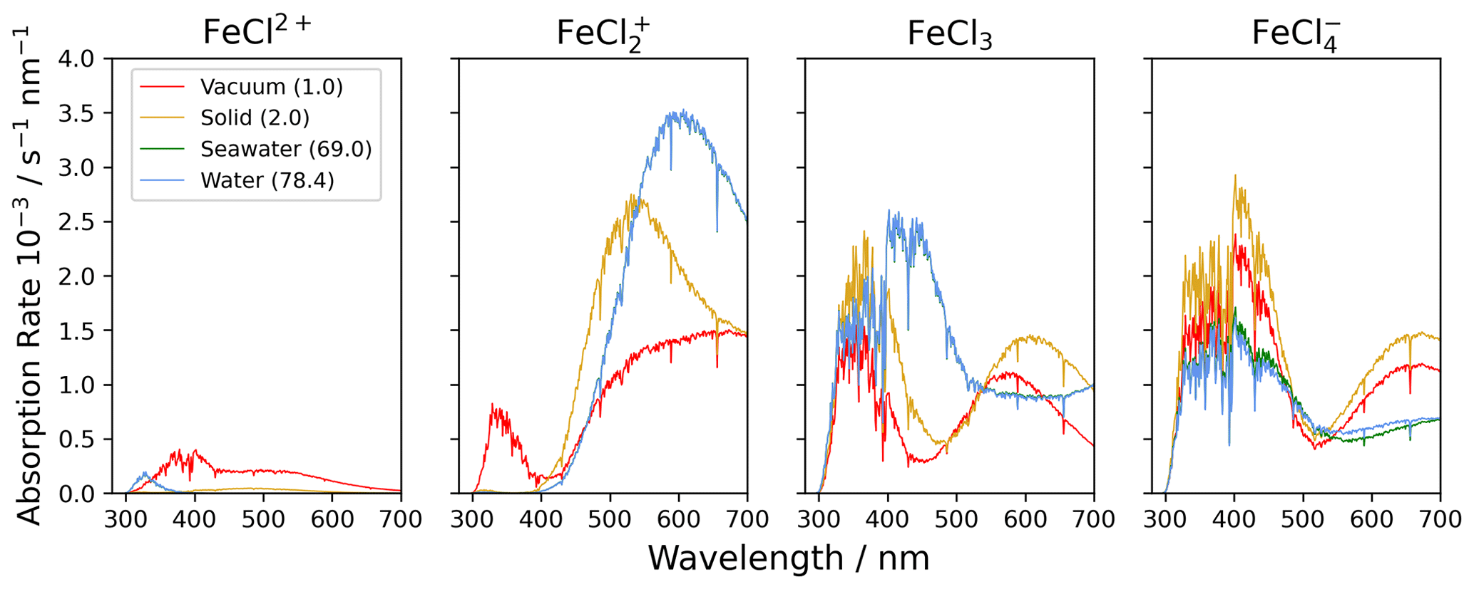
Figure 7 The absorption rate of FeCl²⁺, FeCl${}_{\mathrm{2}}^{+}$, FeCl₃, and FeCl${}_{\mathrm{4}}^{-}$ in vacuum (1.0), solid FeCl₃ (2.0), seawater (69.0), and water (78.4). The value in parentheses shows the relative permittivity of the solute. The absorption is calculated using the CAM-B3LYP/6-311++G(d,p) basis set. The spectral actinic flux is calculated using the TUV model over the Atlantic Ocean, west of Cabo Verde (18.97° N, 39.12° W, date 18 July 2022 at 12:00 LT) (Madronich et al., 2002).

Using the calculated UV-Vis spectra, the actinic flux, and the quantum yield function, the photolysis spectra of FeCl²⁺, FeCl${}_{\mathrm{2}}^{+}$, FeCl₃, and FeCl${}_{\mathrm{4}}^{-}$ are calculated (see Fig. 7). Each of these species absorb at visible wavelengths, which has not been described previously. The modeled result for seawater (green) is almost identical to the result for water (blue); the two spectra overlap in the figure. The lowest absorption rates are calculated for FeCl²⁺, where all rates are below 0.5 × 10⁻³ s⁻¹ nm⁻¹ for all four solvents. The AEM scenarios found FeCl²⁺ to be the second most abundant iron(III) chloride species. Its role becomes less important, however, when the absorption spectrum is considered in addition to the chromophore's concentration.

FeCl${}_{\mathrm{2}}^{+}$ in vacuum absorbs from 300 to 700 nm, whereas solid, seawater, and aqueous FeCl${}_{\mathrm{2}}^{+}$ absorb in the range of 400 to 700 nm. FeCl${}_{\mathrm{2}}^{+}$ in water and seawater have the highest absorption rates of the investigated species, 3.5 × 10⁻³ s⁻¹ nm⁻¹. The AEM scenarios found FeCl${}_{\mathrm{2}}^{+}$ to be the dominant iron(III) chloride species, and when the absorption spectrum is considered in combination with concentration, we conclude that FeCl${}_{\mathrm{2}}^{+}$ is the important chromophore for the catalytic, photo-oxidative conversion of chloride to chlorine in aqueous environments.

In the model, the absorption rates of FeCl₃ in seawater and water have a maximum of 2.6 × 10⁻³ s⁻¹ nm⁻¹ at 402 nm. Similar trends are calculated for FeCl${}_{\mathrm{4}}^{-}$, where the solid has a maximum at 400 nm of 2.8 × 10⁻³ s⁻¹ nm⁻¹. The absorptions in vacuum and solid have similar trends for both FeCl₃ and FeCl${}_{\mathrm{4}}^{-}$.

Visible light does not necessarily provide enough energy for the iron(III) chlorides to dissociate, and a transition state analysis can assist in the estimation of the energy thresholds. In Fig. 8, the energy thresholds for photodissociation yielding a chlorine radical are shown for the four iron(III) chloride species FeCl²⁺, FeCl${}_{\mathrm{2}}^{+}$, FeCl₃, and FeCl${}_{\mathrm{4}}^{-}$. The photon energy is given (in kJ mol⁻¹) and converted to a photon wavelength in nanometers so that it can be related to the solar spectrum. Near the Earth's surface, the actinic flux spectrum becomes negligible at wavelengths shorter than 300 nm (Harnung and Johnson, 2012). This threshold is shown in the figure with a yellow line.

Figure 8 shows FeCl²⁺ as the only species to have an energy threshold corresponding to a wavelength shorter than 300 nm for solid, seawater, and water, and so this species cannot be dissociated by near-surface solar excitation. According to the model, FeCl${}_{\mathrm{2}}^{+}$ has energy thresholds for solid, seawater, and water at 611, 603, and 605 nm, respectively. The highest absorption rates for FeCl${}_{\mathrm{2}}^{+}$ are in the region of 500 to 700 nm (see Fig. 7); thus these thresholds very likely impact the photolysis rate.

According to the transition state model, FeCl₃ is the only species that can be photolyzed by all visible wavelengths and even into the near-infrared for any of the solvents. For FeCl${}_{\mathrm{4}}^{-}$, the only sunlight-limiting energy threshold is in vacuum at 573 nm. However, as FeCl${}_{\mathrm{4}}^{-}$ absorbs at wavelengths shorter than this threshold, sunlight will dissociate this species under vacuum conditions. Sunlight at the surface has photons with enough energy for the dissociation of FeCl${}_{\mathrm{2}}^{+}$, FeCl₃, and FeCl${}_{\mathrm{4}}^{-}$.

General trends in Fig. 8 show vacuum to be an outlier that either has a higher or lower energy threshold than solid, seawater, and water. Therefore, solvent effects play an important role when estimating the energy thresholds and absorption rates of the dissociation of these iron(III) chloride species.

Figure 8 Energy thresholds for photodissociation, yielding a chlorine radical calculated with CAM-B3LYP/6-311++G(d,p). The sunlight photolysis rate cut-off is illustrated in yellow. The relative permittivity for the solutes is given in parentheses.

Table 3 Integrated absorption rates (s⁻¹ × 10⁻³). “Full” is integrated from 280 to 700 nm, as displayed in Fig. 7. “Cut-off” is integrated from 280 nm to the dissociation energy threshold in Fig. 8. The deviation is calculated between the full and the cut-off absorption rates.

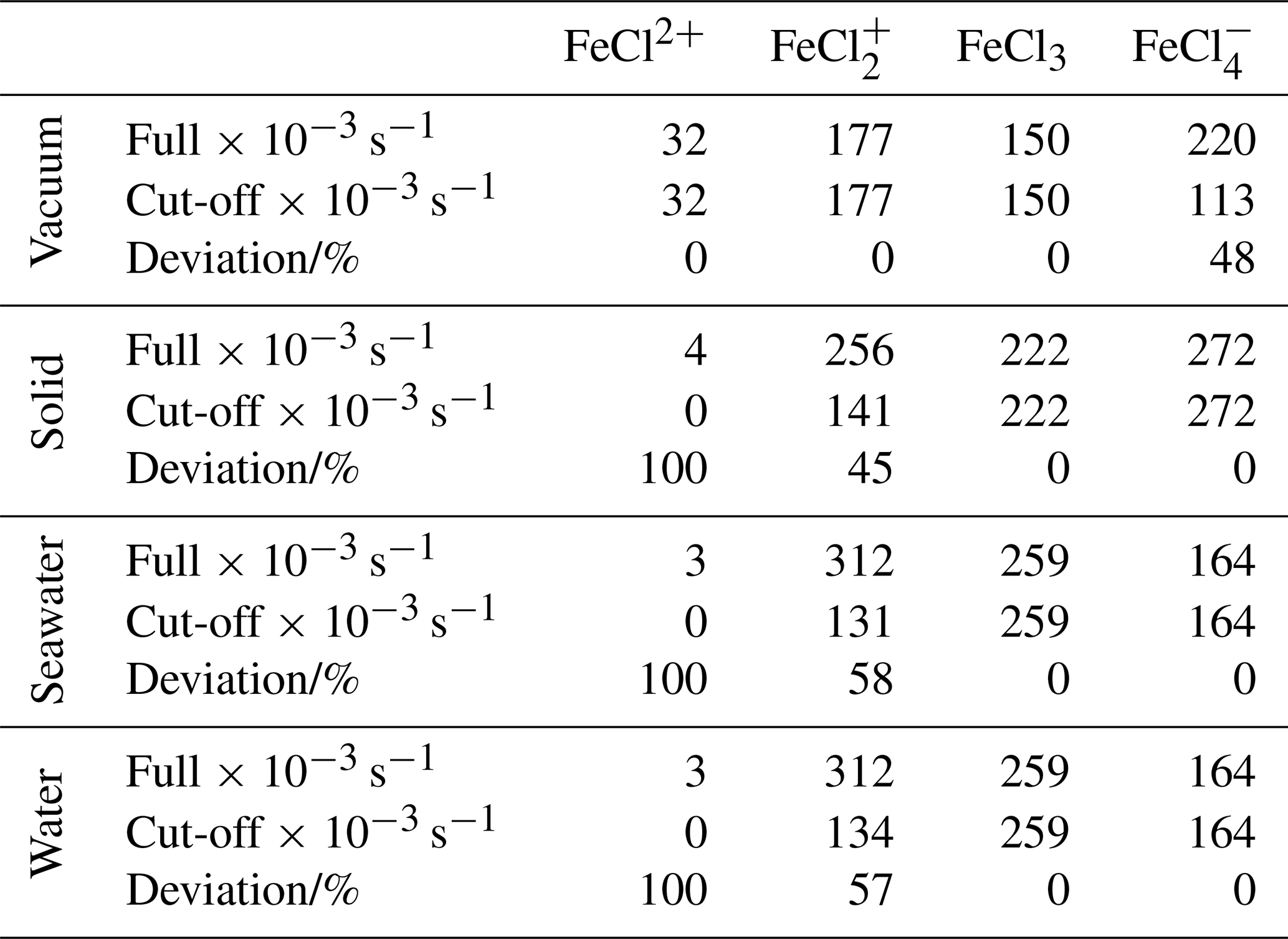
To relate the absorption rates and the energy dissociation threshold, the integrated absorption rates are listed in Table 3. The integrated absorption rate is integrated from 280 to 700 nm, as seen in Fig. 7. The cut-off is integrated from 280 nm to the dissociation energy threshold regarding each species, as seen in Fig. 8. The deviation between full and cut-off is listed in percentages for each species as a measure of the cut-off impact.

As listed in Table 3, FeCl²⁺ has full absorption rates of 32, 4, 3, and 3 s⁻¹ in a vacuum, solid, seawater, and water, respectively. This species generally has the lowest integrated absorption rates, which decrease significantly from vacuum to solid, seawater, and water. When the energy dissociation threshold is included, the integrated absorption rates for solid, seawater, and water decrease to zero.

FeCl${}_{\mathrm{2}}^{+}$ has full absorption rates of 177, 256, 312, and 312 s⁻¹ in vacuum, solid, seawater, and water, respectively. Including the cut-off significantly decreases the absorption rates by 45 %, 58 %, and 57 % for solid, seawater and water, respectively.

FeCl₃ has full absorption rates of 150, 222, 259, and 259 s⁻¹ in vacuum, solid, seawater, and water, respectively. FeCl₃ is the only species that does not have sunlight-limiting energy thresholds; hence, the full and cut-off rates are identical. Furthermore, FeCl₃ has a higher cut-off absorption rate for seawater and water than the other species, which increases the importance of this species.

FeCl${}_{\mathrm{4}}^{-}$ has full absorption rates of 220, 272, 164, and 164 s⁻¹ in vacuum, solid, seawater, and water, respectively. The rates significantly decrease from vacuum to seawater and water. However, including the cut-off significantly decreases the rate in vacuum by 48 %, whereas the rate in water and seawater is unaffected and is consequently faster than the rate in vacuum.

Including the sunlight-limiting energy thresholds, FeCl₃ is the species that has the fastest integrated absorption rates in seawater and water of 259 and 259 s⁻¹, respectively. Across all species, seawater and water have virtually identical rates, which further confirms that quantum calculations made in water can be used to evaluate behavior in seawater.

3.3 Laboratory study

The change in measured methane concentration was used as a proxy for chlorine radical production, as shown in Reaction (R17).

$$\begin{array}{}\text{(R17)}& {\mathrm{CH}}_{\mathrm{4}}+\mathrm{Cl}\cdot \rightleftharpoons {\mathrm{CH}}_{\mathrm{3}}\cdot +\mathrm{HCl}\end{array}$$

The x axis in Fig. 9 is ordered according to the center wavelength of the bandpass filter used in the experiments, where “none” indicates that no bandpass filter was used. The spectral irradiance for the bandpass filters is displayed in Fig. 4.

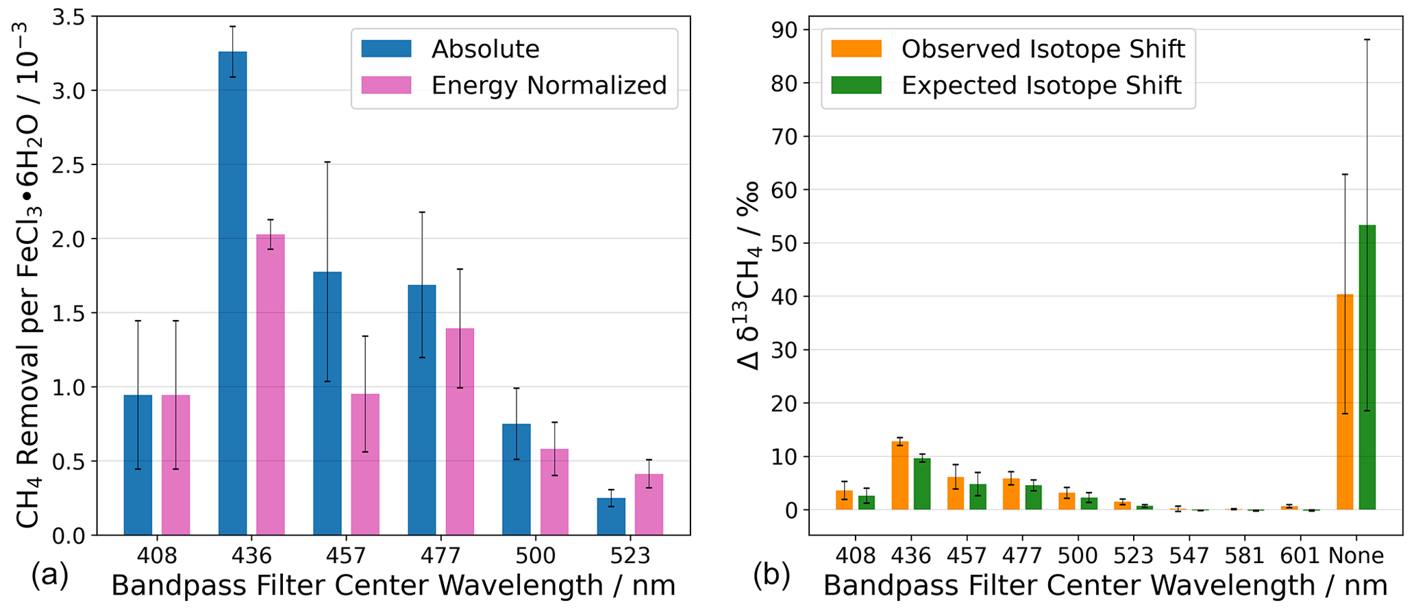
Figure 9 (a) Chlorine generation measured as methane removal for photo-excitation in a series of wavelength intervals defined by bandpass filters. Without a bandpass filter, the absolute CH₄ removal was $\mathrm{10.4}\times {\mathrm{10}}^{-\mathrm{3}}$ CH₄ molecules per FeCl₃ ⋅ 6H₂O molecule. (b) The change in the abundance of ¹³C is shown as Δδ¹³CH₄. The term “none” indicates that no bandpass filter was used during the experiment. Steady-state calculations of Cl are shown in Appendix Sect. A6. The error bars represent the standard deviation.

The absolute and energy-normalized methane removal is shown in Fig. 9 (left) in units of CH₄ molecules per FeCl₃⋅ 6H₂O molecule. The energy normalization was calculated for the absolute removal at 408 nm and the integrated spectral irradiance for each bandpass filter. As the bandpass filters do not have the same wavelength width or energy throughput (Fig. 4), the energy normalization contradicts this effect.

The largest average methane removal occurs at 436 nm. At this wavelength, the removal corresponds to 3.3 × 10⁻³ and 2.0 × 10⁻³ CH₄ per FeCl₃⋅ 6H₂O for absolute and energy-normalized removal, respectively. This means that chlorine generation is small relative to the iron chloride reservoir in the sample. The lowest average methane removal occurs at 523 nm, 0.3 × 10⁻³, and 0.8 × 10⁻³ CH₄ per FeCl₃⋅ 6H₂O for absolute and energy-normalized removal, respectively.

The reaction of methane with chlorine is highly fractionating, and an increase in δ¹³CH₄ would suggest that chlorine is the oxidizing agent and not a different oxidation pathway, e.g., hydroxyl radicals. The abundance of ¹³C in CH₄, measured as δ¹³CH₄, is measured during the experiments with the Picarro G2201-i and is shown in Fig. 9 (right) as the change in the delta value.

A chlorine steady-state (Cl SS) concentration was calculated from the observed CH₄ removal (seen in Fig. 9, left) to derive the concentration of chlorine required to remove an amount of methane (the Cl SS calculation equations are shown in Appendix Sect. A6). The expected δ¹³CH₄ was calculated using the SS Cl concentration with the rate constants for the chlorine oxidation of ¹²CH₄ and ¹³CH₄. The expected δ¹³CH₄ value is shown in green, together with the measured change in the delta value, in Fig. 9b.

Oxidation of methane by OH radicals results in a fractionation 17 times smaller than for the methane, namely the Cl reaction (Saueressig et al., 2001, 1995). A lower-observed-than-expected change in the delta value would indicate an additional removal pathway with a lower kinetic isotope effect (e.g., OH). The observed and expected Δδ¹³CH₄ values are equal to within the experimental uncertainties, except for the experiment made using the 436 nm bandpass filter, which is just outside the mutual uncertainties; we think that this was an anomaly due to a calibration offset. Figure 9b shows a clear correlation between the expected and the observed δ¹³CH₄, indicating that chlorine is the oxidizing agent throughout all experiments.

4 Conclusions

In this work, we have presented a detailed description of the photolysis of iron(III) chlorides in aerosols. Modeling, quantum chemical calculations, and laboratory experiments have provided crucial insight into how iron(III) chloride chromophores behave in aqueous solutions under varying conditions of pH.

Three AEM scenarios were built to describe the speciation of the iron chlorides and the competition inhibiting their formation from hydroxide, sulfate, and other seawater ions. The results show that iron(III) chlorides are the dominant forms of iron at pH < 4.0, and iron(III) hydroxides at pH above this. The addition of sulfate decreased the abundance of FeCl${}_{\mathrm{2}}^{+}$ by up to 40 %. The other seawater species we tested did not have a significant effect. The speciation of FeCl²⁺ and FeCl${}_{\mathrm{2}}^{+}$ changes by up to 70 % over the temperature range of 0 to 100 °C.

Quantum chemical calculations made using the density functional theory method CAM-B3LYP/6-311++G(d,p) were used to investigate FeCl²⁺, FeCl${}_{\mathrm{2}}^{+}$, FeCl₃, and FeCl${}_{\mathrm{4}}^{-}$. Solvent effects for vacuum, solid, seawater, and water were included, using the PCM model and relative permittivities. The four iron chloride species all showed the ability to absorb light in the visible spectrum, and the absorptions in seawater and water are virtually identical. Dissociation energy thresholds were found using transition state calculations to evaluate the energy when a chlorine atom leaves the system. For FeCl²⁺, FeCl${}_{\mathrm{2}}^{+}$, and FeCl${}_{\mathrm{4}}^{-}$, the inclusion of the energy threshold significantly decreased the absorption rates. FeCl₃ was the only species without sunlight-limiting energy thresholds in any solvent. In water, FeCl₃ has the fastest integrated absorption rate of 259 × 10⁻³ s⁻¹, and FeCl²⁺ had the overall slowest rate.

We examined the photolysis of solid FeCl₃⋅6H₂O in nine wavelength intervals, using bandpass filters with center wavelengths ranging from 408 to 601 nm. The maximum methane removal was observed for the 436 nm bandpass filter to be 2.0 × 10⁻³ CH₄ molecules per FeCl₃⋅ 6H₂O, whereas the removal efficiency without a bandpass filter was 10.4 × 10⁻³ CH₄ molecules per FeCl₃⋅6H₂O, including energy normalization. No statistically significant methane removal was observed at wavelengths longer than 523 nm. The observed Δδ¹³CH₄ concluded that methane is oxidized by chlorine and not OH. Maximum chlorine production was found at an excitation wavelength of around 436 nm.

We conclude that the catalytic efficiency of the iron chloride mechanism will be constrained by several environmental variables. The pH of the system plays an important role and affects the abundance of the FeCl${}_n^{\mathrm{3}-n}$ chromophores. Fenton oxidation of Fe(II) to Fe(III) will result in the production of base, which is countered by the absorption of environmental acids like HCl, H₂SO₄, HNO₃, and organic acids. The concentration of chloride also impacts the abundance and distribution of the FeCl${}_n^{\mathrm{3}-n}$ chromophores and will be affected by equilibrium with atmospheric humidity and the emission and re-absorption of HCl. The presence of anions other than Cl⁻, such as sulfate and fluoride, may reduce the availability of Fe(III) for chloride chromophores.

Further research is needed in order to explore the catalytic efficiency of ionic iron and chlorine recycling under the many different conditions in the troposphere and marine boundary layer before the iron chloride mechanism can be considered a potential climate intervention.

Appendix A: Additional methods

A1 Aqueous equilibrium model: species added manually to the Visual MINTEQ database

Table A1 Thermodynamic data for species added to the MINTEQ models. The values were calculated from data by Tagirov et al. (2000). Molar weight (M_w), equilibrium constant (log(K)), and change in enthalpy (ΔH) are shown.

A2 Geometries of iron(III) chlorides

Table A2 Geometries of minima and TS for FeCl²⁺. TS and relative permittivities are given in parentheses. The TS is not optimized if not given otherwise. The Lennard-Jones (LJ) potential is given. Values are given in Ångströms (Å).

Table A3 Geometries of minima and TS for FeCl${}_{\mathrm{2}}^{+}$. TS and relative permittivities are given in parentheses. The TS is not optimized if not otherwise indicated. The Lennard-Jones (LJ) parameters are given in Ångströms (Å).

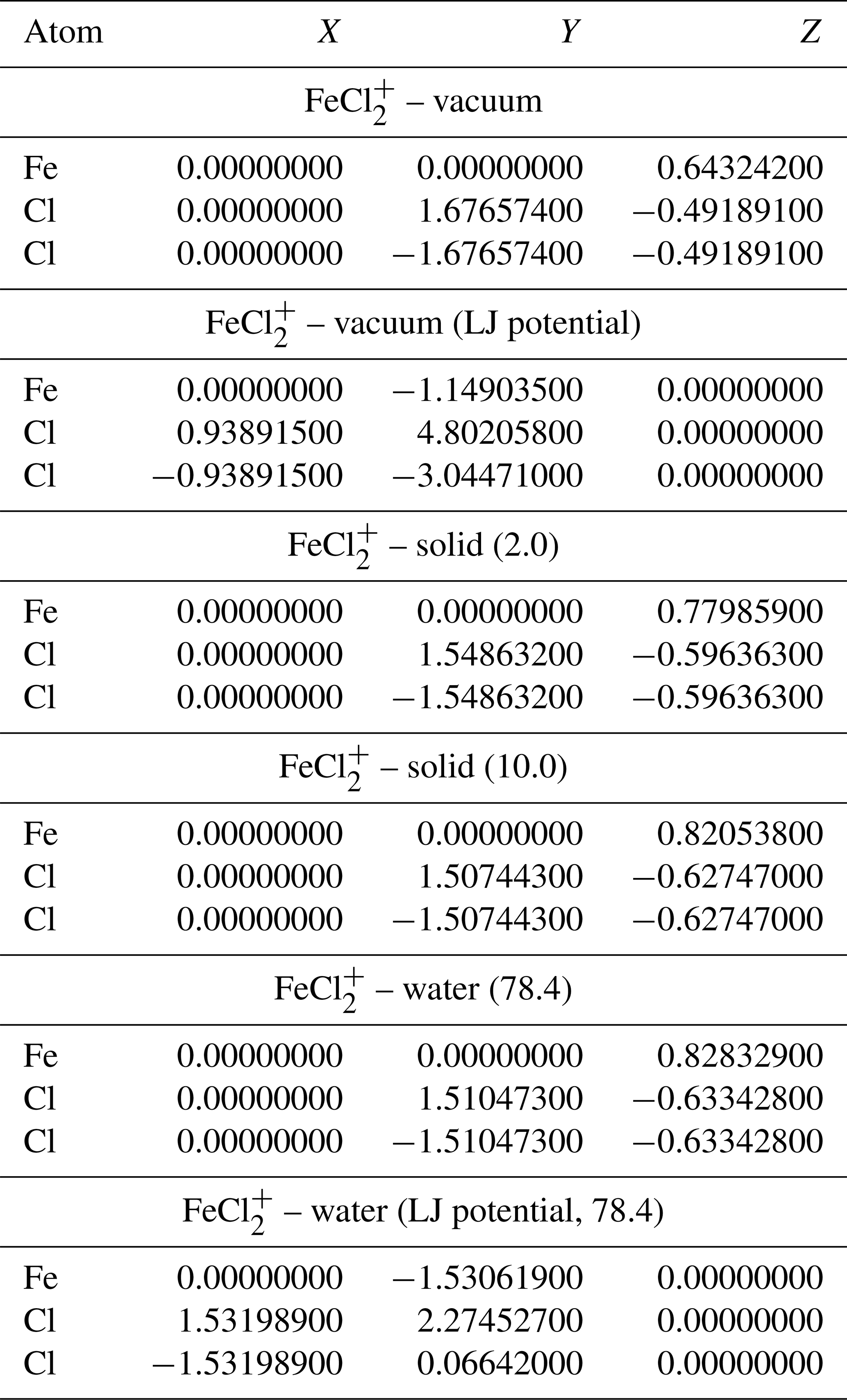
Table A4 Geometries of minima and TS for FeCl₃. TS and relative permittivities are given in parentheses. The TS is not optimized if not otherwise indicated. Values are given in Ångströms (Å).

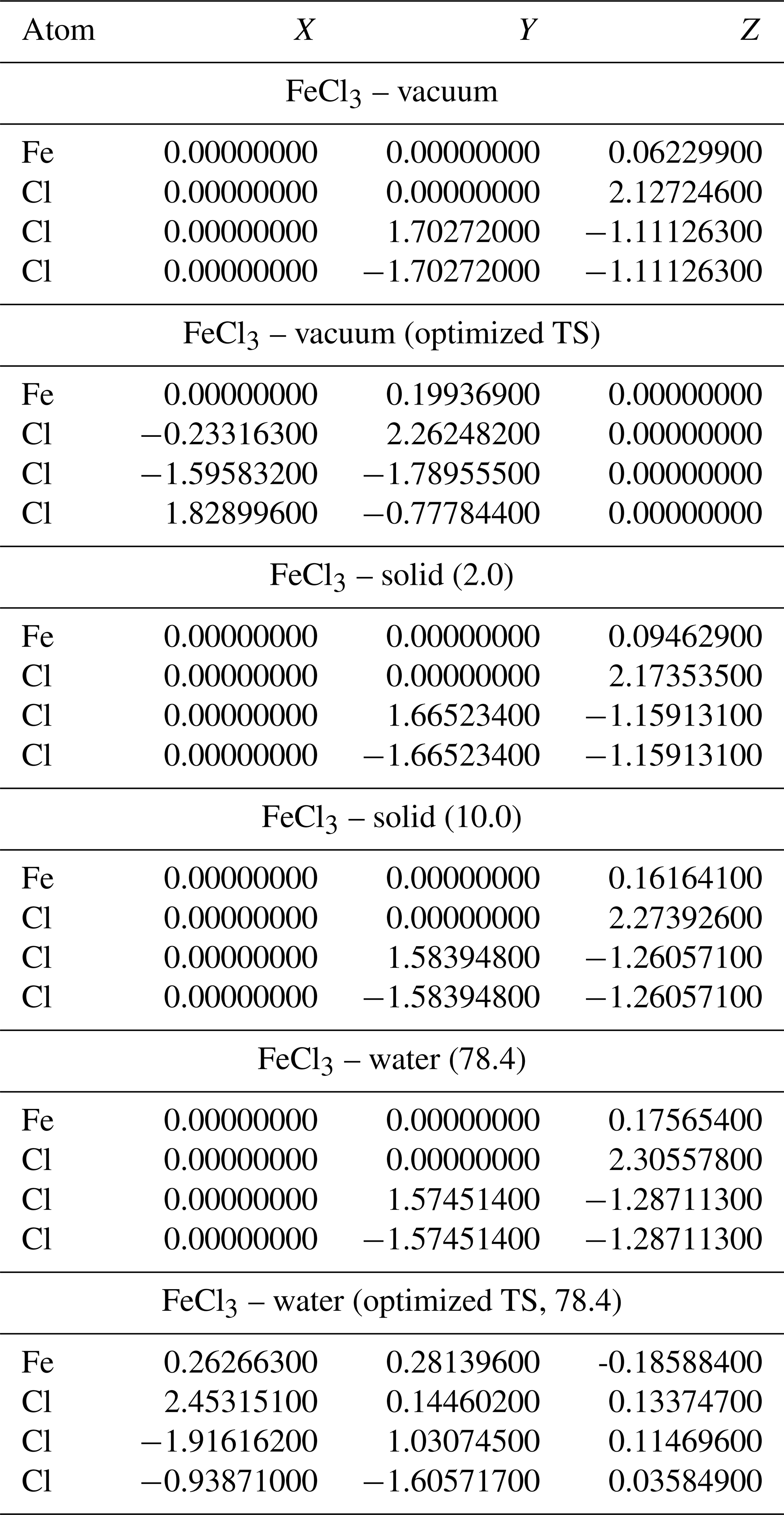
Table A5 Geometries of minima and TS for FeCl${}_{\mathrm{4}}^{-}$. TS and relative permittivities are given in parentheses. The TS is not optimized if not otherwise indicated. Values are given in Ångströms (Å).

Figure A1 Overview of the experimental procedure. Data are retrieved during the three gray highlighted steps. Abbreviations are cold trap (CT), active carbon trap (AC).

A3 Experimental procedure

When the experimental procedure begins, the system is opened between the active carbon trap and the two measuring instruments. While the system is open, the flow is increased, and an overpressure vent is closed to flush the system. A FeCl₃⋅6H₂O sample of 20 mg is now measured in a 10 mL beaker on a fine scale. The sample chamber is cleaned with Milli-Q water on some paper and wiped again with dry paper. The beaker is placed in the sample chamber, and the chamber is closed. Two O-rings ensure a tight closure of the sample chamber. While the system is open, the cold trap is heated for 5 min to flush condensed species out of the system. The active carbon trap is heated for 20 min to release the captured CO₂. The sample chamber is heated simultaneously with the active carbon trap to minimize the temperature difference in the sample chamber when the xenon lamp is turned on. After the heating processes, the flow is decreased by opening the over-pressure vent, and the system is closed. There is now flow through the whole system. During the process of closing the system, the CO₂ and H₂O concentrations are recorded by the Picarro instrument to ensure that the active carbon trap works properly. Methane is now introduced with a syringe to the nitrogen flow. The methane concentration in the system rises to 200 to 400 ppm, and the four-port valve is closed at around 150 ppm. Initiating the methane is controlled live with the Axetris instrument. After the looping process is started, the methane concentration is monitored to ensure that it stabilizes at around 95 ppm. After approximately 5 min, the stability test begins. Due to a small under-pressure state in the system, the presence of a possible leak is quantified by spraying pure methane from a syringe at joints, seals, and so on and observing whether the methane concentration in the system increases. After the system has passed the stability test, the cold trap, bandpass filter, fan, and the UV LED are initiated. The two instruments are both slightly sensitive to temperature, and “leak rate 1” is therefore initiated 5 min after the cold trap is introduced to measure stability. The next step is recording the leak rate over 10 min before illumination. The xenon lamp is turned on for exactly 15 min, and the second leak rate is measured over the following 10 min. One experiment has now ended, and the procedure is repeated with a new sample of FeCl₃⋅6H₂O. The different bandpass filters and light sources are discussed in Sect. 2.3. Each of the 10 bandpass filters was used for three experiments.

A4 Light sources used in the experiments

The xenon lamp, bandpass filters, and sample chamber were placed according to the experimental setup when the irradiance was measured. The chamber setup with measurements can be seen in Fig. A3. The Ocean Optics spectrometer was placed at a distance, according to the bottom of the chamber, to estimate the light exposure for the sample. A calibration was used for the Ocean Optics spectrometer, using the standard manual and light source from Ocean Optics (DH-2000, UV-Vis-NIR calibration light source). The irradiance of the UV LED is shown in Fig. A2.

Figure A2 Light source spectra. The UV LED was a Luminus SST-10-UV Surface Mount LED lamp. The spectrum is recorded by an Ocean Optics Flame-S Miniature UV-Vis-NIR spectrometer and a fiber optic cable with a diameter of 600 µm before and after the chamber.

A5 The sample chamber setup and measurements

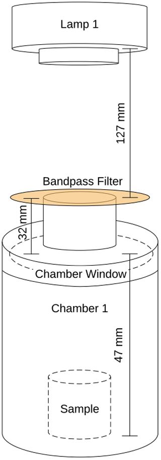
Figure A3 Measurements of the sample chamber setup during the experiments, including the Ocean Optics spectrometer analysis. The sample chamber had a volume of 0.36 L.

A6 Calculation of steady-state chlorine atom concentration and nominal δ¹³CH₄

The steady-state concentration of chlorine atoms is calculated with the assumption of a constant source and sink of chlorine. The decay of methane can be described as a pseudo-first-order reaction in Eq. (AR1):

$$\begin{array}{}\text{(AR1)}& {\text{CH}}_{\mathrm{4}}\left(t\right)={\text{CH}}_{\mathrm{4}}\left(\mathrm{0}\right)\times e^{-rt},\end{array}$$

where t is the time, and r is the first-order loss rate in Eq. (AR2). k(¹²CH₄) is the rate constant of the ¹²CH₄ and Cl reaction, and [Cl]_ss is the chlorine concentration.

$$\begin{array}{}\text{(AR2)}& r=k\left({}^{\mathrm{12}}{\text{CH}}_{\mathrm{4}}\right)\times [\text{Cl}{]}_{\mathrm{ss}}\end{array}$$

The Cl SS concentration is isolated and used to calculate the expected isotope shift. The kinetic isotope effect α is used to define the isotopic fractionation ϵ (Johnson et al., 2002):

$$\begin{array}{}\text{(AR3)}& {\displaystyle }\mathit{\alpha }={\displaystyle \frac{k{(}^{\mathrm{12}}{\text{CH}}_{\mathrm{4}})}{k{(}^{\mathrm{13}}{\text{CH}}_{\mathrm{4}})}}\text{(AR4)}& {\displaystyle }\mathit{ϵ}=\mathit{\alpha }-\mathrm{1}.\end{array}$$

The final isotopic enrichment δ is calculated based on the enrichment of the starting material, δ₀, ϵ, and the extent of reaction, f:

$$\begin{array}{}\text{(AR5)}& {\displaystyle }\mathit{\delta }={\mathit{\delta }}_{\mathrm{0}}+\mathit{ϵ}\cdot \ln \left(f\right).\end{array}$$

Appendix B: Additional results

B1 Ab initio calculations: FeCl₃

Figure B1 Absorption of FeCl₃ calculated with CAM-B3LYP/6-311++G(d,p). Solid (2.0) and solid (10.0) values are estimated to represent the optic and static relative permittivity for the solid state of FeCl₃, respectively.

B2 All aqueous equilibrium models

Figure B2 Simple, sulfate, and seawater aqueous equilibrium models with a total iron concentration of 9.76 $\times {\mathrm{10}}^{-\mathrm{13}}$ mol kg⁻¹ (Fe_S). The right column is magnified from 0 % to 5 %.

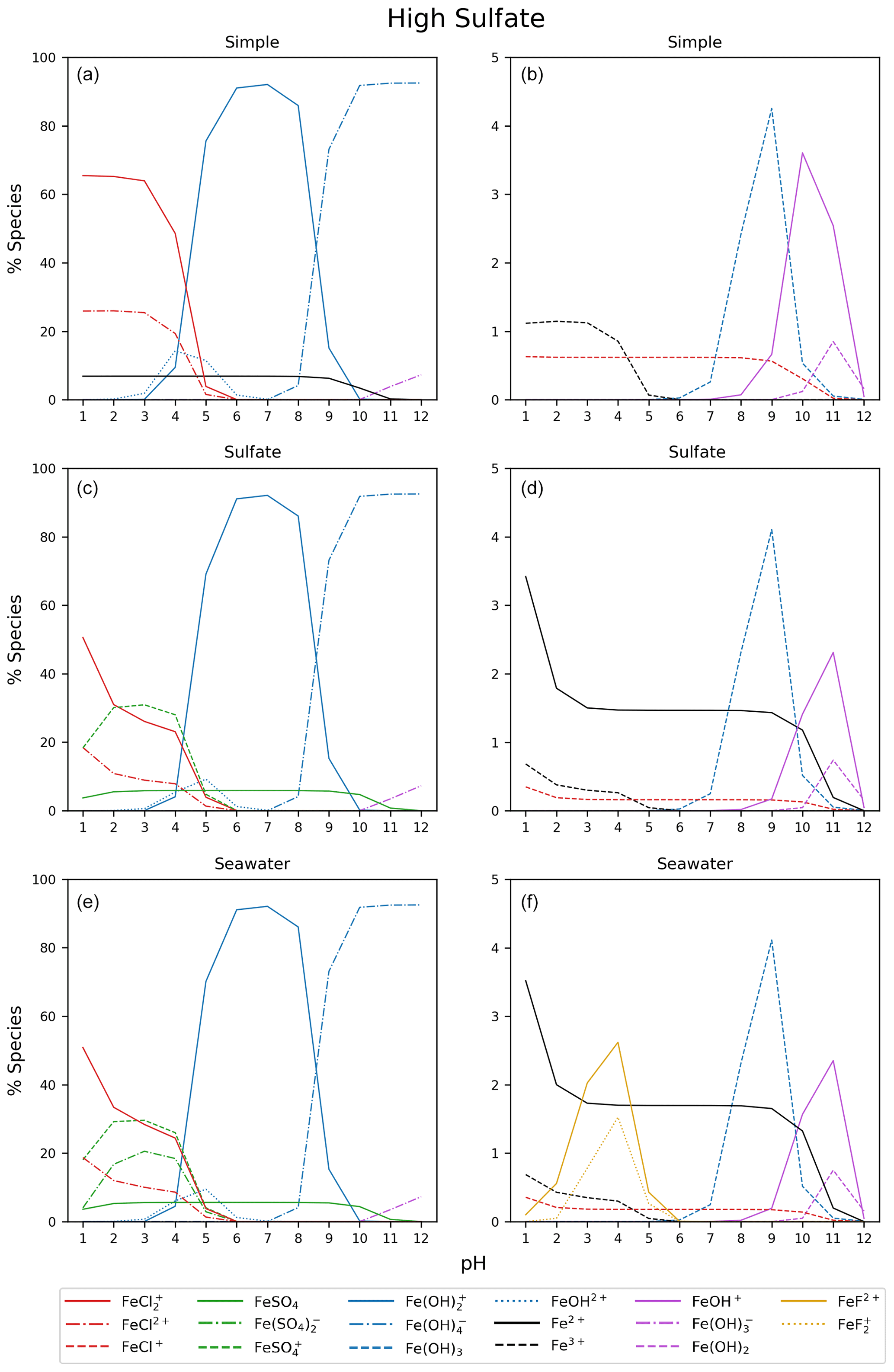
Figure B3 Simple, sulfate, and seawater aqueous equilibrium models with a 10 times higher sulfate concentration (2.82 × 10⁻¹ mol kg⁻¹) and a total iron concentration of 9.76 $\times {\mathrm{10}}^{-\mathrm{13}}$ mol kg⁻¹ (Fe_S). The right column is magnified from 0 % to 5 %.

Figure B4 Simple, sulfate, and seawater aqueous equilibrium models with a total iron concentration of 9.17 $\times {\mathrm{10}}^{-\mathrm{4}}$ mol kg⁻¹ (Fe_A). The right column is magnified from 0 % to 5 %.