Global fields of daily accumulation-mode particle number concentrations using in situ observations, reanalysis data, and machine learning

Accurate global estimates of accumulation-mode particle number concentrations (N₁₀₀) are essential for understanding aerosol–cloud interactions and their climate effects and for improving Earth system models. However, traditional methods relying on sparse in situ measurements lack comprehensive coverage, and indirect satellite retrievals have limited sensitivity in the relevant size range. To overcome these challenges, we apply machine learning (ML) techniques – multiple linear regression (MLR) and eXtreme Gradient Boosting (XGB) – to generate daily global N₁₀₀ fields using in situ measurements as target variables and reanalysis data from the Copernicus Atmosphere Monitoring Service (CAMS) and ERA5 as predictor variables. Our cross-validation showed that ML models captured N₁₀₀ concentrations well in environments well-represented in the training set, with over 70 % of daily estimates being within a factor of 1.5 of observations. However, performance declines in underrepresented regions and conditions, such as in clean and remote environments, including marine, tropical, and polar regions, underscoring the need for more diverse observations. The most important predictors for N₁₀₀ in the ML models were aerosol-phase sulfate and gas-phase ammonia concentrations, followed by carbon monoxide and sulfur dioxide. Although black carbon and organic matter showed the highest feature importance values, their opposing signs in the MLR model coefficients suggest that their effects largely offset each other’s contributions to the N₁₀₀ estimate. By directly linking estimates to in situ measurements, our ML approach provides valuable insights into the global distribution of N₁₀₀ and serves as a complementary tool for evaluating Earth system model outputs and advancing the understanding of aerosol processes and their role in the climate system.

1 Introduction

Accumulation-mode particles are aerosol particles ranging from 100 to 1000 nm in diameter. They can be emitted directly in this size range from various natural and anthropogenic sources or form through the growth of particles either emitted in smaller sizes or formed by atmospheric new particle formation (e.g., Morawska et al., 1999). In the atmosphere, accumulation-mode particles play a critical role in the climate due to their influence on cloud properties and their interaction with atmospheric radiation (Forster et al., 2021).

Cloud formation occurs when an air mass becomes supersaturated, leading to the condensation of water vapor on aerosol particles known as cloud condensation nuclei (CCN), forming cloud droplets (Boucher et al., 2013). Whether a particle can act as CCN at a given supersaturation depends on its composition and size (e.g., McFiggans et al., 2006; Andreae and Rosenfeld, 2008). Particles around 100 nm in diameter are generally large enough to activate as CCN under typical atmospheric conditions regardless of their chemical composition (Dusek et al., 2006; Kerminen et al., 2012; Pöhlker et al., 2021), making the number concentrations of accumulation-mode particles a good estimate for CCN-active particles. Aerosol particles can influence the radiative budget in both direct and indirect ways. The number concentration of CCN-active particles affects the cloud’s properties, for example, cloud albedo, cloud liquid-water path, cloud lifetime, and precipitation properties (e.g., Twomey, 1977; Albrecht, 1989; Forster et al., 2021; Stier et al., 2024). Additionally, because aerosol particles alter the transmittance of radiation in the atmosphere, they can modify the atmospheric temperature profile, impacting the evaporation and condensation processes in the clouds (Forster et al., 2021). Due to the complexity of these interactions, aerosol–cloud interactions remain the largest source of uncertainty in the radiative forcing estimates and future climate projections (Forster et al., 2021).

Understanding the global distribution of accumulation-mode particle number concentrations is essential for improving our understanding of CCN and, therefore, aerosol–cloud interactions. For example, to reliably assess aerosol effects on clouds, global CCN concentrations need to be captured within a factor of 1.5 of their true values (Rosenfeld et al., 2014). However, obtaining such accuracy with measurements on a global scale is challenging. Although in situ measurements of both CCN and accumulation-mode particle number concentrations are available and crucial for understanding spatial variation, they have limited spatial and temporal coverage (Rosenfeld et al., 2014; Schmale et al., 2018). As a result, global observations rely heavily on satellite remote sensing, which introduces its own set of challenges (e.g., Rosenfeld et al., 2014; Bellouin et al., 2020; Quaas et al., 2020). For example, satellites cannot directly observe the aerosol particle number concentrations. Instead, they often rely on indirect retrievals, like radiation extinction-related variables such as aerosol optical depth (AOD) or aerosol index (AI). Inferring number concentrations from these retrievals is challenging because they relate to the entire columnar burden of particles in the atmosphere and are sensitive to other variables, including relative humidity and aerosol particle size. Moreover, satellites cannot detect aerosol loadings beneath clouds, making it difficult to obtain data under the conditions where these measurements would be most needed.

Accumulation-mode particle and CCN number concentrations also pose challenges for Earth system models (ESMs). Accurately modeling aerosol growth from small particles to the accumulation-mode size range requires detailed numerical descriptions of complex aerosol dynamics within ESMs (Blichner et al., 2021). This task is both challenging and computationally expensive, leading to simplified physical representations in ESMs, adversely affecting their accuracy. Many ESMs employ bulk mass aerosol schemes without direct particle number concentration calculations (e.g., Yu et al., 2022). If particle number size distributions are represented in the ESMs, they are typically described with modal aerosol schemes, where distributions are represented by several log-normal modes (e.g., Mulcahy et al., 2020; Blichner et al., 2021; van Noije et al., 2021). However, this method involves a priori assumptions about the size distribution that often inaccurately reflect the true size distributions and thus alter the flow of particles growing from one mode to another (Blichner et al., 2021; Bergman et al., 2012; Korhola et al., 2014). These issues can be avoided by using sectional schemes, where size distributions are represented by size bins, but these are more computationally expensive (Blichner et al., 2021).

Given the challenges of directly measuring accumulation-mode particle and CCN concentrations, as well as the limitations of the ESMs, there is a clear need to develop alternative estimation methods. One such method is the recent work by Block et al. (2024), who derived global CCN concentrations using aerosol mass mixing ratios from CAMS reanalysis data (CAMS data are discussed further in Sect. 3.2). These aerosol mass concentrations, constrained by satellite-retrieved AOD, were converted into aerosol number size distributions based on estimated size distributions for each aerosol species. They then applied modified kappa–Köhler theory to calculate the number of particles that activate into CCN at specific supersaturation levels. Their approach provides valuable insights into global CCN concentrations at different supersaturations, constrained by the satellite observations assimilated into CAMS reanalysis data. However, it does not incorporate direct CCN or particle number measurements and relies solely on CAMS reanalysis data.

Nair and Yu (2020) presented an alternative approach utilizing machine learning (ML) to estimate CCN concentrations. They selected 46 sites across the globe and employed a chemical transport model to calculate CCN concentrations along with various predictors, including aerosol, chemical, and meteorological variables at these locations. This dataset formed the basis for training a random forest regression model, which was then evaluated using CCN observations from the Southern Great Plains (USA) measurement station. Although the method relied primarily on modeled CCN concentrations and predictors, it demonstrated the potential of ML techniques for estimating aerosol number concentrations. A follow-up study utilized a similar approach and estimated particle number concentrations (diameters of 1.2–120 nm) using a random forest regression model (Yu et al., 2022).

Another machine learning application that has gained popularity in atmospheric sciences in recent years is extending observations from measurement stations to larger geographic areas. This method has been quite commonly employed for estimating PM_2.5 and other air pollutant concentrations across local and regional scales (e.g., Ma et al., 2019; Di et al., 2019; Kim et al., 2021; Wang et al., 2022, 2023; Yu et al., 2023). Some methods focus on extrapolating measurements using solely the target measurements from measurement stations with no additional predictors. For example, Ma et al. (2019) utilized a neural-network-based spatial–temporal extrapolation method to estimate PM_2.5 concentrations in the state of Washington (USA). However, in most cases, the ML models are trained to estimate the concentrations based on a range of widely available variables, including other air quality measurements, meteorological data, satellite retrievals, geographical and land use information, reanalysis datasets, and outputs from chemical transport models.

In this study, we employ ML techniques to bridge the gap between localized in situ measurements of accumulation-mode particle concentrations and the global scale. We train two ML models – a multiple linear regression model and an eXtreme Gradient Boosted model (described in Sect. 2.1) – using in situ measurements of N₁₀₀ as the target variable and reanalysis variables from the CAMS and ERA5 datasets as predictors (described in Sect. 3). These models generate daily number concentration fields for particles with dry diameters larger than 100 nm (N₁₀₀). Sect. 4 details our methods for training the ML models and assessing the model performance both at the measurement stations and outside of them. Once trained, we use these ML models to generate daily global N₁₀₀ fields N₁₀₀ for 2013. We also investigate the reliability of the global ML models across different regions based on the influence predictor variables have on the models and how the multiple linear regression (MLR) and eXtreme Gradient Boosting (XGB) model fields differ.

2 Background on machine learning methods

This section contains a brief overview of the methods and the two different ML models we used in this study to estimate N₁₀₀. Further reading on these methods can be found, for example, in Kuhn and Johnson (2013). The more detailed description of how we applied these techniques is in Sect. 4.

2.1 ML models

Multiple linear regression (MLR) is a simple yet effective method that extends ordinary least squares regression to model the relationship between multiple predictor variables and a single target variable (e.g., Kuhn and Johnson, 2013). It assumes a linear relationship between the set of predictors and the target. The MLR model finds a linear equation consisting of coefficient terms for each predictor variable and a constant term (intercept) to minimize the sum of squared residuals between the predicted and observed values.

The method of eXtreme Gradient Boosting (XGB) combines a tree-based ensemble method with gradient boosting (Chen and Guestrin, 2016). In simple terms, XGB trains sequentially weak predictive estimators (decision trees) that, at each step, aim to correct the errors of the previous estimators. The final estimate is calculated as the sum of the decision tree estimates. The number of trees can typically be between 100 and 1000. XGB is used for both regression and classification tasks. Here, we used it for regression with the squared error as the loss function.

We chose these two ML models because they complement each other well. MLR is a simple, interpretable model that provides insights into the relationships between predictors and the target variable through the coefficients. It can also extrapolate beyond the range of values in the training data, at least if the relationship with the target variable and the covariates is linear. In contrast, XGB is well-suited to complex, non-linear data and interactions but is more computationally intensive and difficult to interpret. XGB is also more limited in its ability to extrapolate beyond the range of values in the training data as it predicts constant values far outside the training data. By using both MLR and XGB, we can compare two fundamentally different ML methods. The differences in the estimates produced by the ML models may shed light on the global ML model performance, which is otherwise difficult to assess.

2.2 ML training and evaluation process

2.2.1 Training, validation, and holdout sets

A typical supervised learning process, such as regression, as discussed here, involves two main steps: model training and performance evaluation. A portion of the full dataset, called the training set, is used to train the model. During training, the model learns from both the target and predictor variables in the training set, adjusting its internal parameters to capture their relationship.

Once the model is trained, its performance is evaluated with a portion of the full dataset that is separate from the training set. In the testing phase, the trained model receives only the predictor variables and generates estimates for the target variable. These estimates are then compared against the observed target values to assess model performance. To prevent data leakage and ensure reliable model performance assessment, the datasets used for training and testing the model must remain independent.

To maintain the independence of the datasets used for training and testing the model, the model performance of the final ML model is typically evaluated with a dedicated dataset called the holdout set. This subset of the full dataset is set aside from the training data at the beginning of the analysis and is reserved solely for testing the final ML model at the end of the analysis. The allocation of data between training and holdout sets depends on the specific application. This includes how many data are assigned to each set and which data points are selected for training versus testing. When data are limited, allocation must be done carefully to ensure that both sets remain representative. In some cases, it may be preferable to forgo data splitting and to train the model on all available data. In these cases, resampling methods such as cross-validation (CV) can be used to evaluate model performance using only the training data.

2.2.2 K-fold cross-validation

In CV, the original training set is further divided into smaller groups, namely a new training set and a validation set, the latter of which is now used to evaluate the model performance. We used two types of CV, k-fold CV and spatial CV.

K-fold CV involves dividing the original training set into k groups. One group serves as the validation set, while the remaining groups form the new training set. The model undergoes training and testing iteratively, rotating through each group. The process yields k performance values, and the average of these values is utilized to evaluate the model's performance. The benefit of using CV is that each data point can be used both to train the model and to test its performance while maintaining the separation between the sets to ensure reliability.

Given the spatial structure of our dataset, we complemented traditional k-fold CV with spatial CV. In spatial CV, folds are defined based on geographical information (e.g., Cho et al., 2020; Beigaitė et al., 2022) – in our case, by measurement station. Because data from the same location are autocorrelated, including a station’s data in both the training and validation sets can lead to overly optimistic performance estimates. Spatial CV mitigates this issue by ensuring greater independence between folds because the target station’s own data are not used in training.

2.2.3 Model optimization

CV is also used for model optimization, a step prior to training the final model. This phase involves fine-tuning the model to enhance its performance of the specific task. In our case, optimization included feature selection and hyperparameter tuning.

Feature selection refers to selecting a subset of predictor variables (also known as features) for the ML mode. If the dataset contains predictor variables that correlate with each other, having multiple variables with similar information is redundant. It can also cause overfitting, where the model becomes too tailored to the training data and performs poorly on unseen data, making the models less generalizable. The best practice is selecting only the relevant variables.

Hyperparameters (HPs) are user-defined parameters that control the complexity of the model. Increasing complexity can improve the performance on the training data, but it also increases the risk of overfitting. Tuning HPs is essential to find the right balance between model complexity and generalization ability. MLR does not require HPs in its basic form, while XGB involves several important HPs, such as the number of trees, tree depth, learning rate, and regularization parameters (XGBoost Developers, 2022). To optimize the HPs, we employed grid search, which is a commonly used brute-force method where each hyperparameter is given a range of manually selected values, following which the search iterates over all possible combinations. The search can be repeated multiple times, focusing only on a subset of hyperparameters or using narrowing ranges of values based on previous rounds. We evaluated the performance of each hyperparameter combination using CV and selected the combinations that yielded the best average performance over the validation folds.

2.2.4 Model performance metric

For the performance metric, we used the root mean squared error (RMSE) between the log₁₀-transformed observed N₁₀₀ values and the log₁₀-transformed estimated N₁₀₀ values (RMSE${}_{{\log }_{\mathrm{10}}}$). We used log₁₀-transformed N₁₀₀ values in our analysis because we were interested in capturing the correct order of magnitude rather than the exact N₁₀₀ values. Additionally, RMSE is scale-dependent, resulting in higher errors for higher N₁₀₀ values. Log₁₀ transformation mitigates this issue.

The RMSE${}_{{\log }_{\mathrm{10}}}$ calculated using the training set is referred to as the training error, and the RMSE${}_{{\log }_{\mathrm{10}}}$ calculated with a separate holdout set is referred to as a testing error. A low RMSE${}_{{\log }_{\mathrm{10}}}$ indicates good performance, whereas higher values indicate poorer performance. In this study, we considered the model performance with RMSE${}_{{\log }_{\mathrm{10}}}$ below 0.2 to be excellent (at least 70 % of the estimated values were within a factor of 1.5 in relation to the observed values, i.e., between the observed value divided by a factor of 1.5 and the observed value multiplied by a factor of 1.5), values below 0.3 to be good (at least 50 % of the estimated values were within a factor of 1.5 in relation to the observed values), and values above to be 0.3 poor (below 50 % of the estimated values were within a factor of 1.5 in relation to the observed values).

2.2.5 Feature importance

Interpreting the ML model involves assessing the importance of each variable (also known as features). The estimation of feature importance differs between MLR and XGB models. In MLR models, importance is determined by the coefficients of the variables. When variables have a similar range of values or are scaled, the absolute value of a coefficient indicates its importance, and the sign (positive or negative) shows whether an increase in the variable leads to an increase or decrease in N₁₀₀. In contrast, XGB models do not have a straightforward method for estimating variable importance; instead, they provide various approaches (XGBoost Developers, 2022). We used the gain method, which evaluates importance based on the accuracy improvement in a branch when a variable is included (XGBoost Developers, 2022).

3 Data description and processing

3.1 Measured N₁₀₀ (target variable)

The dataset contained ground-level in situ N₁₀₀ measurements from 35 measurement stations worldwide (Fig. 1). Depending on the station, the measurements were performed with either a differential mobility particle sizer (DMPS) (Aalto et al., 2001) or a scanning mobility particle sizer (SMPS) (Wiedensohler et al., 2012). The dataset contained sub-hourly N₁₀₀ calculated from the number concentration of particles between 100 nm and the upper limit of the measurement instrument, which varied between 400 nm and 1000 nm (Table 1). Because the number concentration of accumulation-mode particles is typically dominated by particles with diameters well below 400 nm (Leinonen et al., 2022), it is very unlikely that the differing upper limits have a notable impact on our results. Further descriptions of each station, the measurement instrument used, and references are in Table 1.

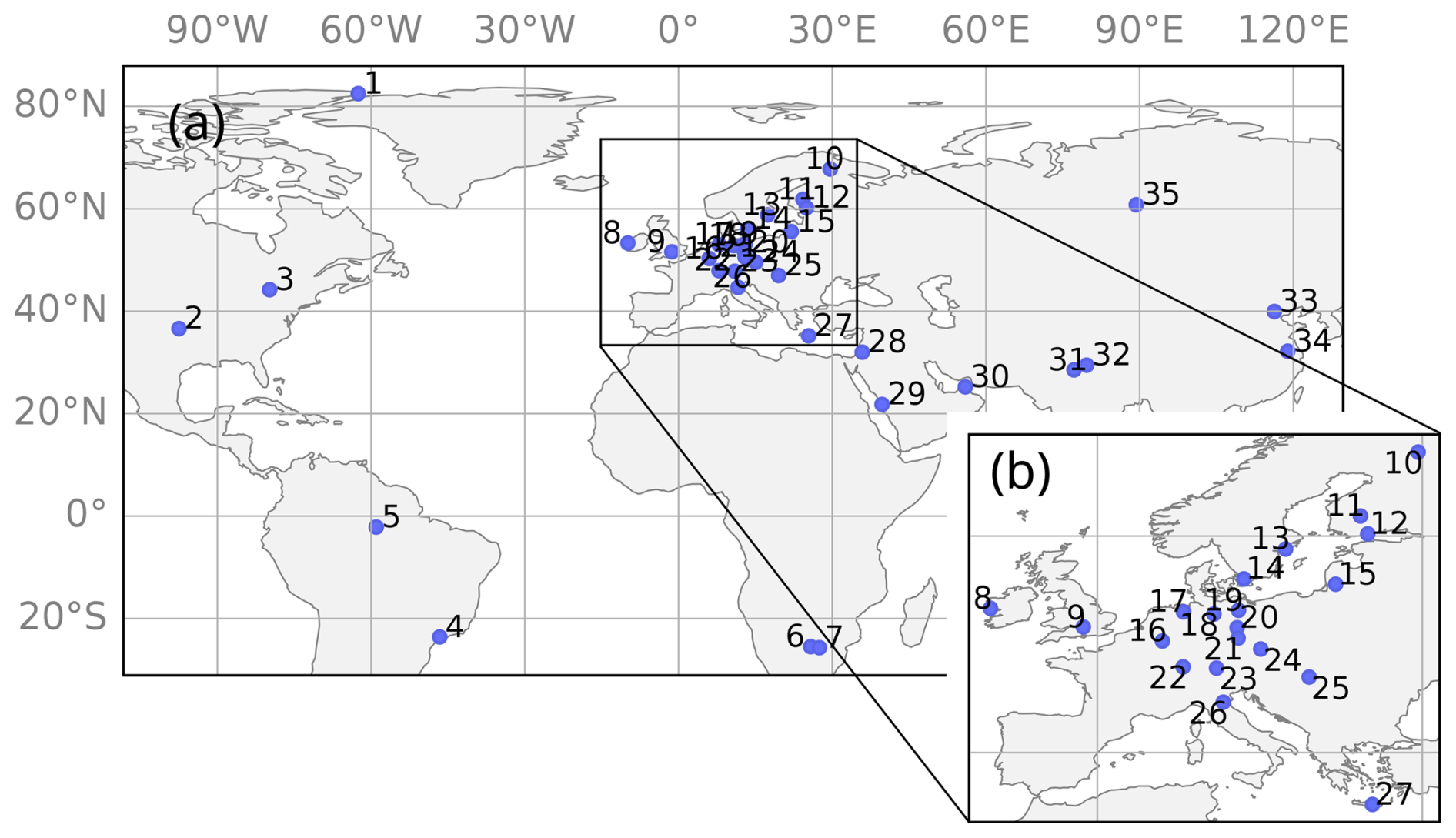
Figure 1 Map of measurement stations. Panel (a) shows the map, and panel (b) shows a zoom-in on Europe. The numbers refer to stations as listed in Table 1.

We separated the measurements into training and holdout sets based on temporal division (discussed further in Sect. 4.1). The training set contained observations from 2003 to 2019, with the specific measurement periods and data availability varying across stations (Fig. 2). The shortest available time series covered 201 d, while the longest extended over 6182 d, altogether comprising 49 490 data points. The holdout set contained N₁₀₀ measurements for 2020–2022. For this time period, we had data from fewer stations, covering only a subset of European stations with, altogether, 9587 data points. The data availability of this testing dataset can be seen in Fig. S1 in the Supplement.

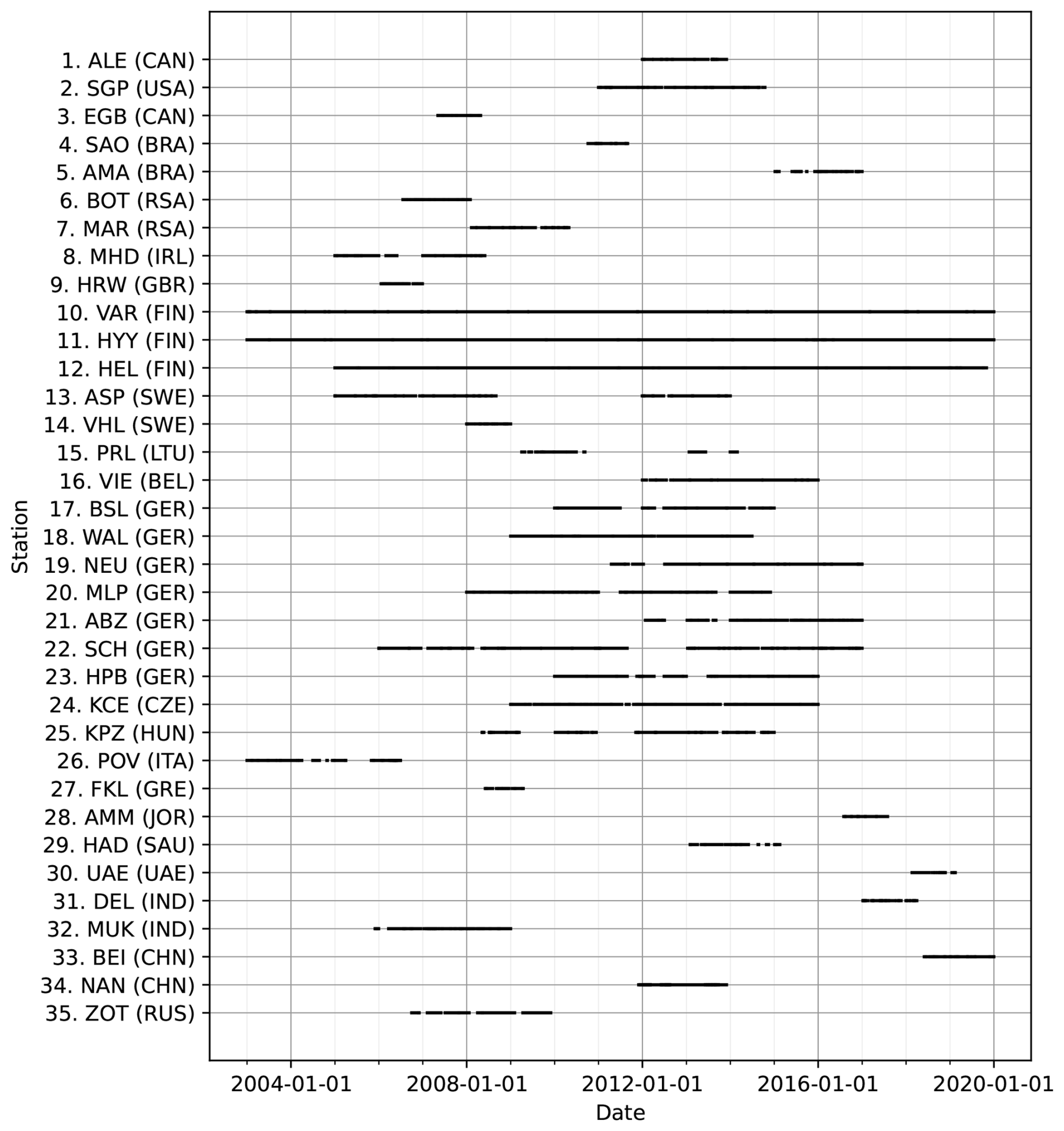
Figure 2 The temporal data availability of N₁₀₀ measurements at different stations in the training set. The station numbers and abbreviations correspond to Table 1.

We processed the N₁₀₀ measurement data by first ensuring all timestamps were in UTC time and then calculating daily averages. To address outliers likely caused by measurement errors, we removed values outside three standard deviations from the station's mean. The observed N₁₀₀ concentrations ranged from a few particles per cubic centimeter to tens of thousands of particles per cubic centimeter. Because the N₁₀₀ concentrations show roughly a log-normal distribution and because our aim was to capture the correct order of magnitude rather than exact N₁₀₀ values, we employed log₁₀ transformation for N₁₀₀.

Leaitch et al. (2013)Marinescu et al. (2019)Pierce et al. (2014)Backman et al. (2012)Andreae et al. (2015)Vakkari et al. (2013)Laakso et al. (2008)O'Connor et al. (2008)Charron et al. (2007)Hari et al. (1994)Hari and Kulmala (2005)Järvi et al. (2009)Tunved and Ström (2019)Kristensson et al. (2008)Mordas et al. (2016)ACTRIS (2024)Asmi et al. (2011)UBA (2013)UBA (2013)Engler et al. (2007)Schladitz et al. (2015)UBA (2013)Birmili et al. (2003)Zíková and Ždímal (2013)Yli-Juuti et al. (2009)Hamed et al. (2007)Kalivitis et al. (2015)Hussein et al. (2019)Lihavainen et al. (2016)Kesti et al. (2022)Gani et al. (2020)Hooda et al. (2018)Liu et al. (2020)Qi et al. (2015)Heintzenberg et al. (2011)

Table 1 List of measurement stations included in this study and their information, including the station number used to identify stations in the figures (No), station full name and country, the abbreviation used in the text, coordinates (latitude, longitude) and altitude above sea level in meters, station environment type, instrumentation, maximum diameter of the measurement, and references. The measurements were conducted either with differential mobility particle sizer (DMPS) or scanning mobility particle sizer (SMPS).

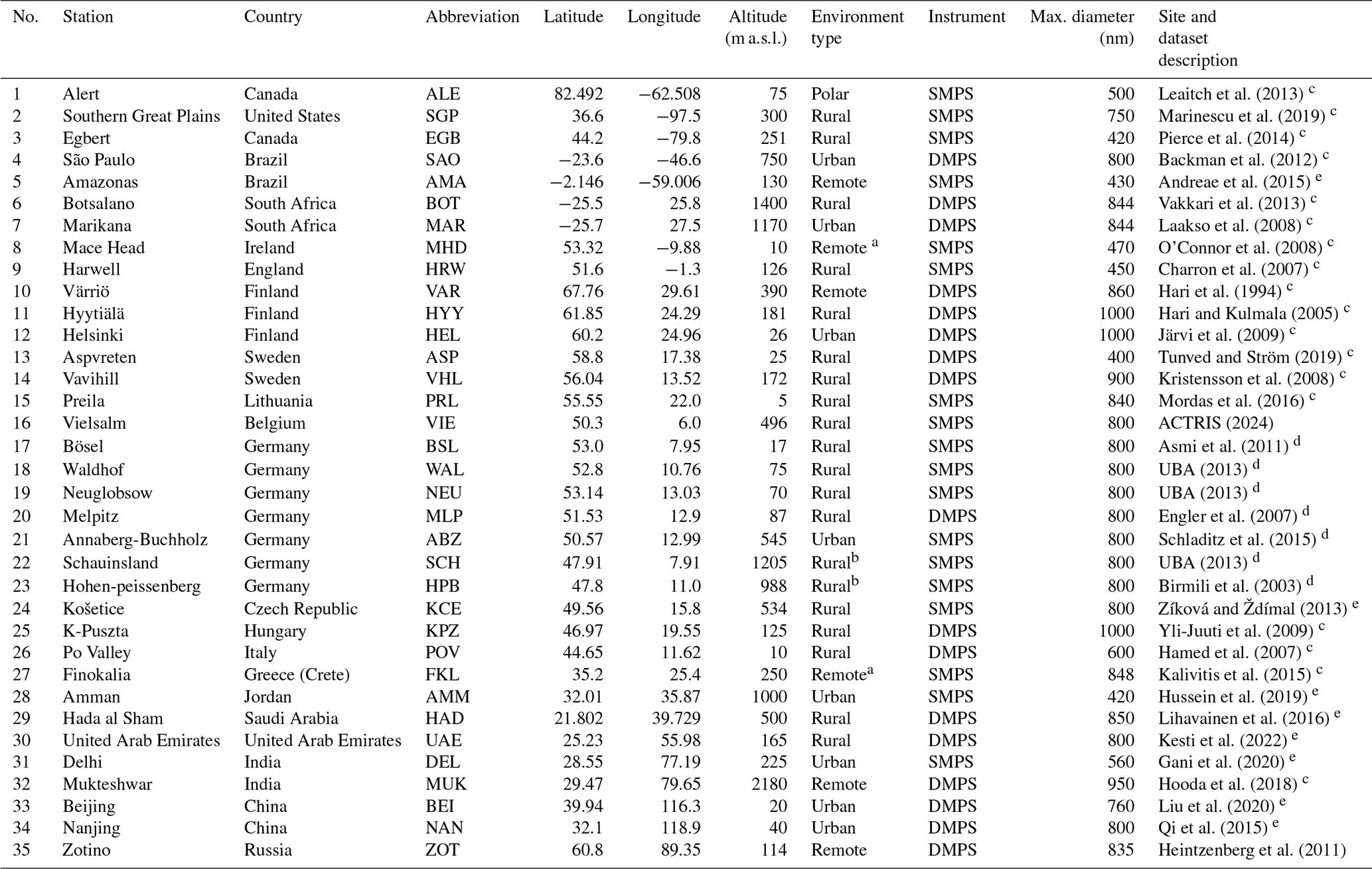
^a Coastal site. ^b Mountain site. ^c Dataset reference: Nieminen et al. (2018). ^d Dataset reference: Birmili et al. (2016). ^e Dataset reference same as measurement site reference.

3.2 Reanalysis data (predictor variables)

Reanalysis data make up a gridded dataset created by assimilating observations from various sources, such as in situ measurements and satellite retrievals, into a numerical weather prediction model. In this study, we used reanalysis variables collected from the Copernicus Atmosphere Monitoring Service (CAMS) “CAMS global reanalysis (EAC4)” dataset (Inness et al., 2019a, b) and the “ERA5 hourly data on single levels from 1940 to present” dataset (Hersbach et al., 2023). Both datasets are generated by the European Centre for Medium-Range Weather Forecasts using the Integrated Forecasting System (IFS) model for numerical weather prediction. CAMS provides global datasets for past atmospheric composition with 3-hourly time resolution and 0.75 × 0.75° spatial resolution. ERA5 offers global datasets for numerous atmospheric variables at an hourly time resolution and 0.25 × 0.25° spatial resolution.

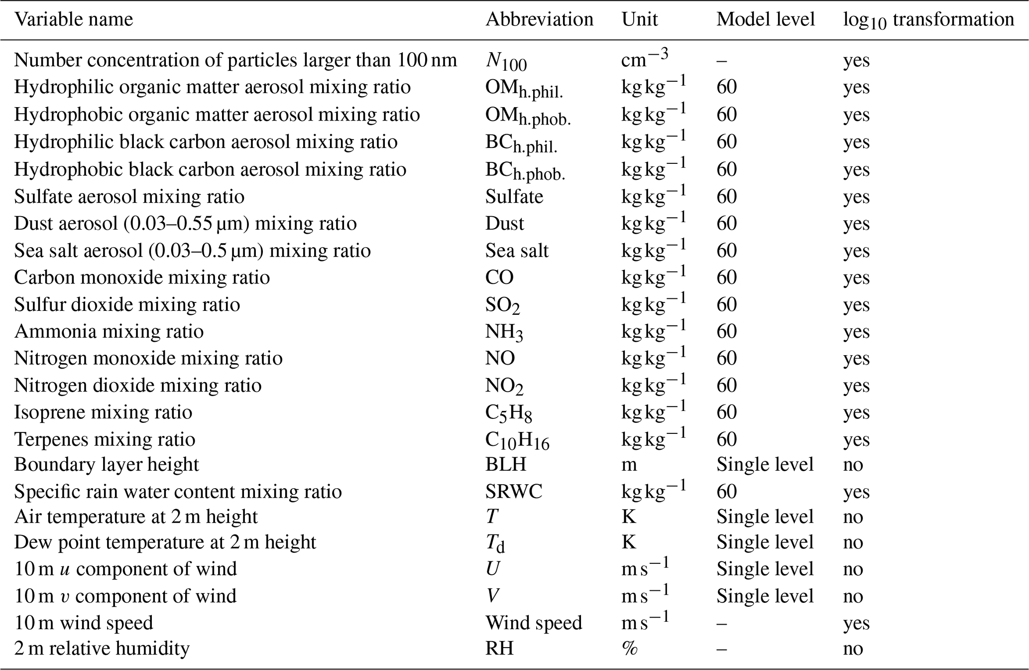
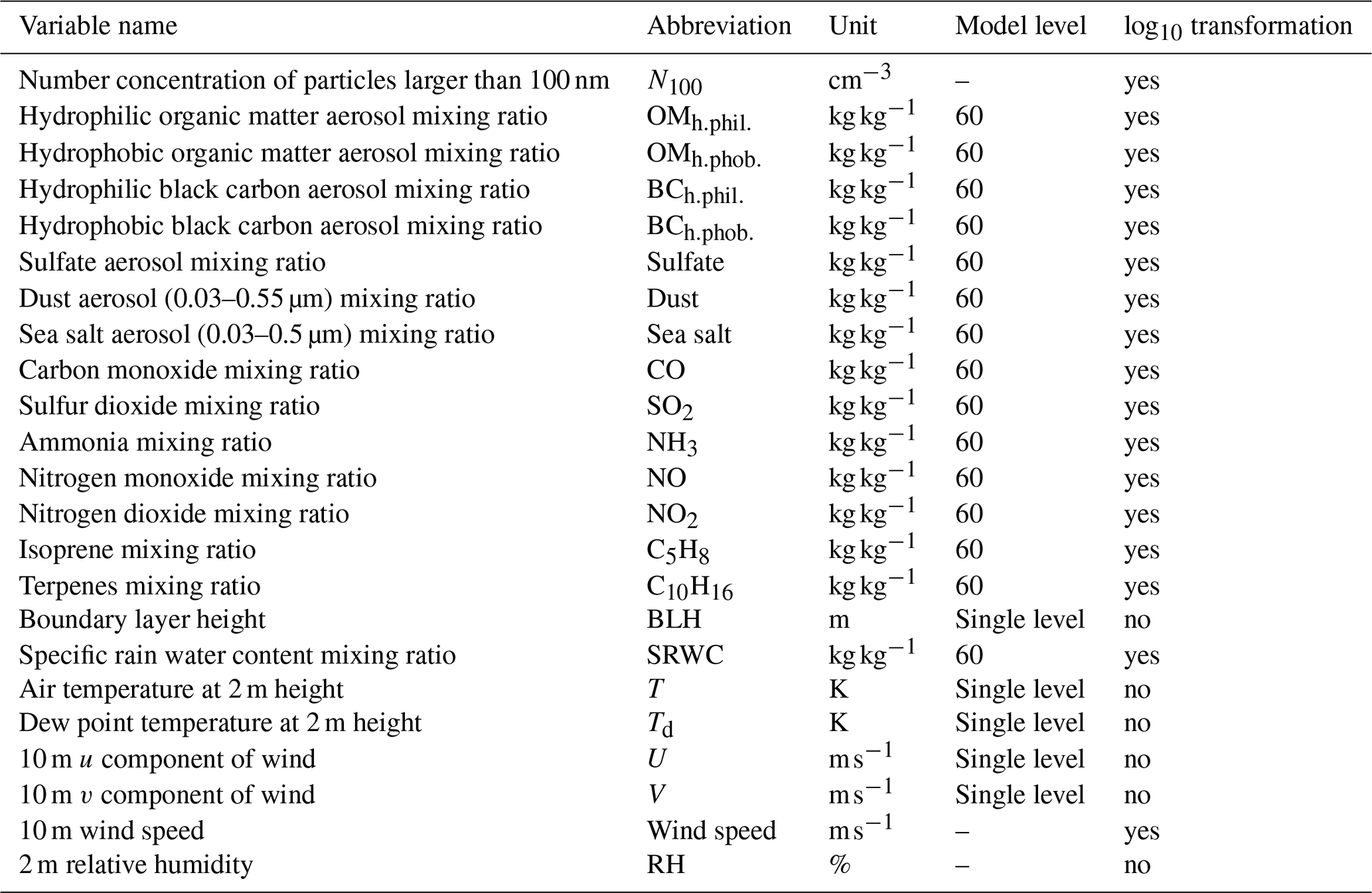
The list of reanalysis variables used as predictors is provided in Table 2. Most variables were sourced from the CAMS dataset, while boundary layer height (BLH) was obtained from the ERA5 dataset. The selected reanalysis variables are known to influence N₁₀₀ either directly or indirectly. The variables with a direct influence relate to primary emissions in the N₁₀₀ size range (black carbon, organic matter in terms of primary organic matter, sulfate aerosol, the smallest size ranges of dust and sea salt aerosol) and their sinks (rain). The variables with an indirect influence either contribute to secondary aerosol formation and, thus, particle growth into the N₁₀₀ size range (sulfur dioxide, ammonia nitrogen monoxide or dioxide, terpenes, isoprene, organic matter in terms of secondary organic aerosol, temperature, relative humidity), affect their transportation and dilution, or indicate general exposure to combustion and biomass burning in the air masses (wind speed, BLH, carbon monoxide). Many of these variables can be related to multiple processes affecting N₁₀₀ concentrations, as discussed in Sect. 5.2.1.

Table 2 Information on the variables used in model training and testing. The table lists variable names, variable abbreviations, variable units, model level of reanalysis data if applicable, and whether the variable was log₁₀ transformed. N₁₀₀ was obtained from measurements. The other variables were from reanalysis data, with boundary layer height from the ERA5 dataset and other reanalysis variables from CAMS reanalysis data. Wind speed and relative humidity were calculated from CAMS variables. The reanalysis variables contained some single-level variables, but most of the variables were multi-level variables, which we downloaded for model level 60, which is 10 m above ground under standard atmospheric conditions.

Reanalysis variables served as predictors in the training and holdout sets. In these sets, we collocated the reanalysis data to the N₁₀₀ measurements by using values interpolated to the point of the measurement station and including only days with observations. For the training set, we selected observations from the period of 2003–2019 and, for the holdout set, observations from the period of 2020–2022. However, the average conditions within a grid cell (up to around 80 km) and even the interpolated values may sometimes fail to represent the single-point measurements due to sub-grid-scale variability in emission sources, meteorology, and topography. For example, if a measurement station is located near strong sources or within a limited high-emission area, such as a city, the grid cell average in the reanalysis data may underestimate concentrations due to dilution over a larger area. We discuss the possible effects of these and other CAMS-variable-related uncertainties in Sect. 5.3 and 5.4.

In addition to the training and holdout sets, we used reanalysis data as input for generating the global N₁₀₀ fields, retrieving the reanalysis data covering the whole globe at a 0.75 × 0.75° resolution for 2013. We chose this year because it had the best availability of observational data for assessing model performance.

For the global fields, we first adjusted the 0.25 × 0.25° resolution of the ERA5 dataset to match the 0.75 × 0.75° resolution of the CAMS dataset by calculating grid cell averages that correspond to the CAMS data grid size. The rest of the analysis proceeded in the same way for all sets. We calculated daily averages for the variables. Additionally, we derived two variables from CAMS data: 2 m relative humidity (RH) and 10 m wind speed (WS). RH was computed from the dew-point temperature and air temperature at 2 m height using the approximation of Alduchov and Eskridge (1996) for saturation vapor pressure. WS was calculated from the 10 m u component and 10 m v component of wind.

Finally, we normalized the reanalysis variables that followed a log-normal distribution by log₁₀ transforming them (Table 2). Some of the variables had minimum values at zero, and, before log₁₀ transforming, we replaced these with the next smallest value of the variable. Additionally, if the log₁₀-transformed value was very low compared to the rest of the values (e.g., 10⁻²⁷), we shifted the minimum value to 10⁻¹⁷. This increase in the minimum value was necessary because we noticed that, in situations when the predictor values were extremely low compared to typical predictor values, it led the MLR model to generate unphysically low N₁₀₀ estimates.

4 Designing and applying training and testing procedures

In this section, we detail how the ML methods described in Sect. 2 were applied in our training and testing process for the ML models. The primary aim of this study was to train global ML models using limited observational data to estimate N₁₀₀ concentrations in areas without measurements. The challenge is not training the global ML models but assessing their performance and reliability outside the measurement stations, which cannot be done with our limited holdout set. Therefore, we designed a methodology incorporating cross-validation and intermediate ML model versions. Although we developed this approach for our specific data, it can be applied to other scientific questions in atmospheric and other fields of science, with similar challenges related to limited spatial observations.

4.1 Training and holdout sets and their limitations

As described in Sect. 3, we allocated the training and holdout sets based on temporal selection using data from the period of 2003–2019 for training the models and data from the period of 2020–2022 for assessing model performance. This division was chosen because 84 % of measurements in our dataset were collected during 2003–2019. Training ML models that can be applied globally required a training set that represented diverse environments and meteorological conditions, ideally covering several seasonal cycles at each location to provide reliable analysis. However, as is often the case in atmospheric sciences, most stations did not have long observational series. Given these constraints, we prioritized the training set robustness over the holdout set representativeness and chose to include only stations with 2020–2022 data for the holdout set. This approach also allowed us to investigate temporal extrapolation, where we assessed model performance at the measurement stations but outside the time period used in training.

The presented train–test split had certain limitations. In addition to excluding many of our measurement stations, the holdout set could not assess global ML model performance outside the locations used for training. This drawback was crucial because our goal was not only to estimate N₁₀₀ at the measurement stations (temporal interpolation and extrapolation) but also to evaluate how well the ML models could predict values in completely new locations (spatial extrapolation). To properly assess spatial extrapolation, we would need a holdout set containing additional stations with sufficiently long time series from different environments. However, long time series of particle number size distributions are not widely available, particularly outside Europe. Therefore, ensuring a wide variety of measurement stations in both training and holdout sets is challenging, and datasets from any additional measurement stations would also improve the training set.

Table 3 Summary of the different intermediate model setups and their train–test splits.

4.2 Intermediate models for inferring global model performance

To address the challenges our dataset posed with regard to training and testing the ML models, we employed CV, which allowed us to maximize data usage by utilizing each data point for both training and testing while maintaining separation between the sets in each CV round. As a result, this method could be applied to all stations regardless of data length. However, utilizing CV had two main limitations.

First, because CV involves evaluating ML models based on the same data used for model optimization, it may overestimate the model performance. To investigate this potential bias, we compared CV performance (training error) with holdout set performance (testing error) at stations where a holdout set was available.

Second, for training the final global ML models, we wanted to maximize the training set representation by using all available data from the period of 2003–2019. This approach precluded the direct use of CV for evaluating the final global ML models. To address this, we calculated testing errors for stations with available holdout sets, but, for the other stations, we relied on an alternative strategy. We trained several intermediate models and assessed their performance with CV to infer global ML model performance. Although using separate ML models for generating estimates and assessing their performance was not ideal, this method utilized our limited data more effectively than reserving either portions of each station’s data or entire station datasets for testing.

We constructed several intermediate models with different setups and corresponding CV train–validation splits (Table 3). The first setup involved single-station models, which we trained and tested using only station-specific data. These provided a simple baseline performance analysis for what our method could achieve. The second setup consisted of station-excluded models, where we utilized spatial CV. We trained station-excluded models with all stations except the target station, which acted as the validation set. This approach provided insight into model performance in locations without measurements. The third setup, station-included models, was similar to the station-excluded models but included a portion of the target station’s data in the training set, allowing a comparative analysis against station-excluded models. Additionally, for illustration purposes, we constructed modified versions of the station-included and station-excluded models to generate a time series for 2013. We discuss the different intermediate model setups in more detail in Sect. 4.4.

We structured the model training and testing procedures into three main parts. First, we defined the training and testing procedures, including data sampling, scaling, feature selection, and hyperparameter tuning, to ensure consistency and reliability across all ML models (Sect. 4.3). Second, we conducted CV analyses for the intermediate models (Sect. 4.4). Finally, we trained the global ML models, assessed feature importance, and produced estimates for 2013 (Sect. 4.5).

4.3 Model optimization and training and validation procedures

4.3.1 Train–validation splits for cross-validation

The first step in the analysis was formulating the CV procedures for the intermediate models and determining how to sample and process the training and validation sets to ensure a balanced contribution from all stations. We modified the conventional k-fold CV method and devised two main variations for splitting the data into training and validation sets. We used these variations and their combinations when training and testing the intermediate models (Table 3).

The first variation, a spatial train–validation split used for spatial CV, treated each measurement station as a group. One station was excluded from the training set, and the model performance was tested based on this excluded (target) station. This version was used to construct the station-excluded models (Table 3).

The second variation employed a temporal train–validation split to ensure that the seasonal cycle was represented in both training and testing. Here, each station’s data were divided into four increments, with 2 weeks being allocated to the training set, 3 d being discarded, 8 d being assigned to the validation set, and another 3 d being discarded. Although discarding days reduced the data availability, it minimized autocorrelation between the training and validation sets, preventing overestimated performance. We typically repeated this process four times, rotating the weeks in the sets.

4.3.2 Balancing the training set

The train–validation splits allowed us to assess the model performance while maintaining representation from all selected stations. However, the data length varied between the stations, with the shortest measurement series covering 201 d (about 6 and a half months), whereas the longest spanned 6182 d (about 17 years) (Fig. 2). As a result, the training sets contained a different number of days from different stations. Training the models without addressing this imbalance could bias the global ML models towards stations with longer time series. To address the issue, we implemented a weight that was inversely proportional to the number of data points in the station. Data points from stations with longer measurement series were assigned a lower weight and shorter series were assigned a higher weight so that all stations had equal influence during training. While this approach sacrificed some benefits of longer measurement series, it preserved all information from these longer datasets and was therefore preferable to sampling only a subset and discarding the rest.

Additionally, most of our stations were situated in Europe (Fig. 1), prompting us to investigate if this Eurocentricity could produce bias in our ML models. We trained models with three different station selection schemes and used cross-validation with a spatial train–validation split to evaluate their performance at stations outside of Europe. The station selection schemes were (1) using all stations, (2) sampling a subset of the European stations, and (3) downweighing the data points from European stations. We separately investigated how the selection scheme affected model performance at European stations and non-European stations. The analysis revealed that using all stations yielded comparable model performance in relation to the two other methods for both European and non-European stations. Training the models with data from all stations in the training set even resulted in better median RMSE${}_{{\log }_{\mathrm{10}}}$, though the improvement was not statistically significant (not shown). Thus, we decided to incorporate data from all stations into our training set.

4.3.3 Feature scaling and selection

An essential part of training the ML models involved processing the predictor variables (features). The variables had different units, and their values differed by several orders of magnitude. Such discrepancies can pose a challenge for ML models, potentially affecting their performance (e.g., Kuhn and Johnson, 2013). Additionally, assessing feature importance with MLR coefficients requires the variables to be scaled. To address this, we centered and scaled the variables – subtracting the mean and dividing by the standard deviation – using a scaling function fitted to the weighted training data. We applied this scaling to both the training and the validation or holdout sets.

We also explored different feature selection approaches but ultimately included all variables in our analysis. We investigated how the model performance was affected by selecting only the most important variables, using only a certain type of variable (aerosol variables, meteorological and gas variables), or combining the strongly correlating variables together. However, reducing the number of variables decreased the model performance, likely because all variables were relevant to at least some of the measurement stations. We confirmed, using adjusted R², that including all variables did not artificially inflate model performance due to the larger number of predictors (not shown). As a result, we chose to include all variables in our analysis.

4.3.4 Hyperparameter tuning

After establishing the other training and testing procedures, we focused on tuning hyperparameters (HPs) for the XGB model. We used a grid search and the spatial train–validation split method for cross-validation to ensure that the tuned HPs generalized across all stations (Table 3). One station, Schauinsland, Germany (SCH), was excluded from HP tuning due to its frequent positioning above the boundary layer during winter (Birmili et al., 2016). Based on the grid search results, we selected parameter combinations that produced strong average RMSE${}_{{\log }_{\mathrm{10}}}$ across cross-validation rounds. When multiple parameter sets performed well, we chose the ones that minimized training time.

One of the hyperparameters we tuned was n_estimators, which sets the number of estimators and, consequently, training rounds during the model training. Even though we tuned this variable, we also chose to use early stopping to avoid overfitting and to save computing resources (e.g., Kuhn and Johnson, 2013). Early stopping evaluates model performance after each training round using a validation set and halts training if no improvement is observed after a set number of iterations. In our case, RMSE${}_{{\log }_{\mathrm{10}}}$ was used as the error metric, and training was stopped if performance did not improve after 10 consecutive rounds.

Throughout our analysis, we used one set of tuned HPs. Originally, we formulated the training and testing procedures with default HPs. After deciding the procedure for training the final global ML models (detailed in Sect. 4.5), we tuned the HPs to align with the final training configuration. The final set of HPs can be found in Table S1. We then revisited the training and testing formulations described above to ensure that the initial conclusions remained valid.

4.4 Assessing model performance with intermediate models

Once we had established the ML model training and testing procedures, we trained and tested the intermediate models and used the results to investigate the model behavior and performance.

4.4.1 Single-station models

As outlined in Sect. 4.2, our first intermediate model setup involved training single-station models for each individual station (Table 3). These models provided insight into how well ML models trained specifically for one station could predict N₁₀₀ at that location, a simpler task compared to modeling global N₁₀₀ variations. We trained and tested the single-station models using CV with the temporal train–validation split: 2 weeks from each month were allocated to the training set, and 8 d were allocated to the validation set, with this being repeated four times with different days rotated in the sets (Table 3). For consistency, we scaled the variables, and, for XGB, we applied early stopping and the tuned global HPs.

Although we considered tuning HPs for individual single-station models, we found that using globally tuned HPs was sufficient. For instance, when evaluating the performance of a single-station model for Alert, Canada (ALE) (a station with unique characteristics because it is located in very clean polar environment), results showed minimal improvement when using station-specific HPs (not shown). To conserve computational resources, we chose to use the global HP set across all single-station models.

Following cross-validation, we analyzed the results to assess the models' performance at each station and between the MLR and XGB models. To verify the reliability of our results, which CV may overestimate, we also evaluated single-station model performance using the holdout set for the stations where it was available.

4.4.2 Station-excluded models

The second intermediate model setup involved station-excluded models, designed to evaluate global model performance in stations not represented in the training data (Table 3). This step was essential for estimating how well the global models could perform in areas without measurements. We employed the spatial train–test split for CV, testing the models using all available data from the target station while training them with data from all other stations. To ensure balanced contributions from each training station, we applied weighting to the data points. We scaled the variables and, for XGB, used tuned hyperparameters and early stopping. We conducted an analysis for both MLR and XGB and compared their performance at each station. Additionally, for stations with available holdout sets, we evaluated the performance of the station-excluded models using these sets.

4.4.3 Station-included and station-excluded model comparison

To assess the impact of including data from the target environment in the training set, we constructed station-included models (Table 3). For CV, we used a combination of spatial and temporal train–validation splits. The training set comprised data from all other stations, along with 2 weeks per month of data from the target station, while the validation set contained 8 d per month from the target station. As with the standard temporal train–validation split, we conducted four CV rounds. We also scaled the variables and used tuned HPs and early stopping for XGB.

Additionally, to enable direct comparison between the station-included and station-excluded models, we created a modified version of the station-excluded models. As before, the training set contained data from all stations except the target station, and the validation set included only data from the target station. However, in this version, the validation set was further restricted to include only the days that matched the temporal validation set (Table 3). This process involved four CV rounds, rotating through different validation sets. The scaling, HPs, and early stopping were applied as before.

4.4.4 Time series analysis

As the final step in assessing model performance, we analyzed the time series generated by the station-excluded and station-included models, comparing them to the observed N₁₀₀ time series. The goal was to demonstrate the potential performance of the final global ML models, both at the measurement stations and in areas without measurements. This analysis was conducted for 2013 as this year had the most comprehensive data availability across different stations.

To generate the estimated N₁₀₀ for this analysis, we followed a procedure similar to the original station-excluded and station-included models (Table 3), with one key modification: the validation sets contained data from only 2013. For the station-excluded models, this involved still using the spatial train–validation split but with the validation set restricted to 2013 data. Similarly, for the station-included models, we continued to apply the combined spatial and temporal train–validation split, but the validation set consisted solely of 2013 data. However, unlike in the previous steps, we did not use cross-validation rounds for the station-included models; instead, we used the first 2 weeks of each month as the training set. For both setups, we scaled the data using the scaling function trained on the training sets, and, for XGB, we applied the tuned HPs and early stopping.

With the station-excluded and station-included models trained and the corresponding validation sets defined, we generated estimates for 2013. The station-excluded models produced continuous time series, while the station-included models generated time series with only an 8 d period for each month, as determined by the validation set. After generating the estimated N₁₀₀ time series, we compared them to the observed measurements.

4.5 Global ML models and N₁₀₀ fields

In the final part of the analysis, we proceeded to train the global ML models, analyze their feature importance, and generate global N₁₀₀ fields for 2013.

We trained the final global ML models with a training set containing all stations, all available data points, and all variables. As before, the data points in the training set were weighed to ensure an equal contribution from all stations to the model training. We also fitted the scaling function with the training data, scaled the variables with it, and saved it to be used as a scaler when generating the global N₁₀₀ fields for 2013. Once the training set was processed, we proceeded to train the global MLR model (MLR_global). For the global XGB model (XGB_global), we followed the same procedure, except with the addition of the tuned hyperparameters and early stopping. Here, it should be noted that, in principle, early stopping requires separate training and validation sets to evaluate when the model performance plateaus. However, given that the global ML model training did not have a train–test split, we instead used the training set for evaluation. Early stopping caused the model training to be interrupted after around 425 training rounds (compared to 900 from our HP tuning), potentially earlier than when it would have occurred with separate sets. Nevertheless, because we had utilized early stopping in the previous analyses to mitigate overfitting and save computing resources, we continued to implement it here.

Once we had trained the MLR_global and XGB_global, we proceeded to analyze how different variables contributed to these models using model-given feature importance.

Finally, to generate the global N₁₀₀ fields for 2013, we utilized the 2013 global reanalysis dataset. After scaling the dataset using the previously fitted scaler, we provided it as input for the MLR_global and XGB_global models and generated daily N₁₀₀ fields for 2013.

We investigated the global ML models' performance both at measurement stations and in areas without measurements. At the measurement stations, we evaluated the global ML models using the holdout set for stations with N₁₀₀ data available between 2020 and 2022. In areas without measurements, we compared the MLR_global and XGB_global fields. We calculated the RMSE${}_{{\log }_{\mathrm{10}}}$ between these estimates for each grid cell, and, if the error value was large, it indicated that the models generated very different estimates for that region, meaning at least one must be inaccurate. Conversely, we could assume that the estimates were more reliable if the models produced similar results. However, even when the models yielded similar results, we could not be certain that the estimates were close to the true N₁₀₀ without actual measurements from those locations. For example, if our reanalysis dataset contained a bias in a particular region, both models could produce similar but erroneous results. Since the comparison between MLR_global and XGB_global fields provided only a rough error estimate, we attempted to develop a more sophisticated method for assessing global performance. However, this effort did not yield results.

5 Results and discussion

5.1 Assessing intermediate model performance

5.1.1 Single-station model performance

The training errors for the single-station models are shown in Fig. 3. While generating these models was not the primary goal of this study, they provided a simpler setting to evaluate our method and to identify potential challenges. Many single-station models achieved RMSE${}_{{\log }_{\mathrm{10}}}$ values below 0.2, and almost all remained under 0.3, indicating that model performance was generally excellent or good.

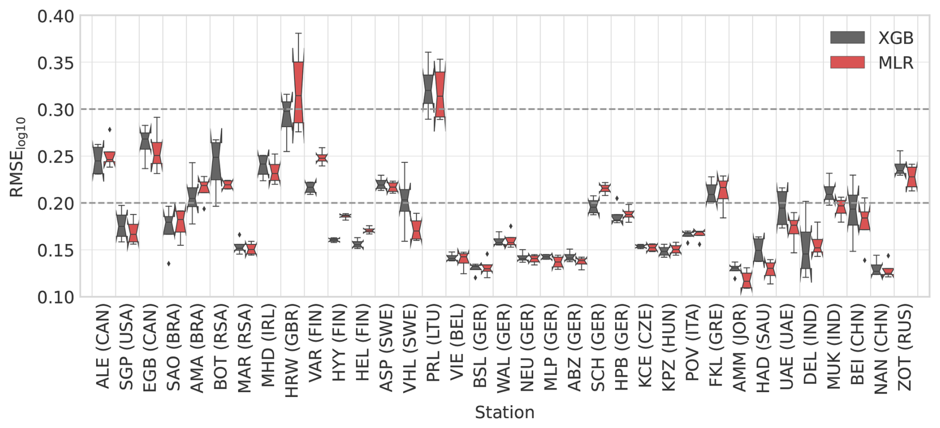
Figure 3 Comparison between training errors (RMSE calculated for log₁₀-transformed concentrations) of the single-station models for one station with XGB and MLR machine learning models. The boxes and whiskers indicate the variation caused by selecting different train–test splits. The boxes show the quartiles, and whiskers show the 1.5 interquartile range of the lower and upper quartile. Data points outside these are considered to be outliers and are marked with individual markers. Additionally, notches in the boxplots indicate the confidence interval of the median. If the notches of two boxes do not overlap, this indicates that the medians are statistically significantly different at the 5 % significance level.

Testing errors for stations with data from the period of 2020–2022 are shown in Fig. 4. As expected, testing errors were slightly higher than training errors, but the overall conclusions remained consistent. These results demonstrate that estimating N₁₀₀ using ML models and reanalysis data is feasible. However, at some stations (e.g., Harwell, United Kingdom, and Preila, Lithuania), model performance was inadequate (RMSE${}_{{\log }_{\mathrm{10}}}>$ 0.3), which we discuss further in Sect. 5.3.

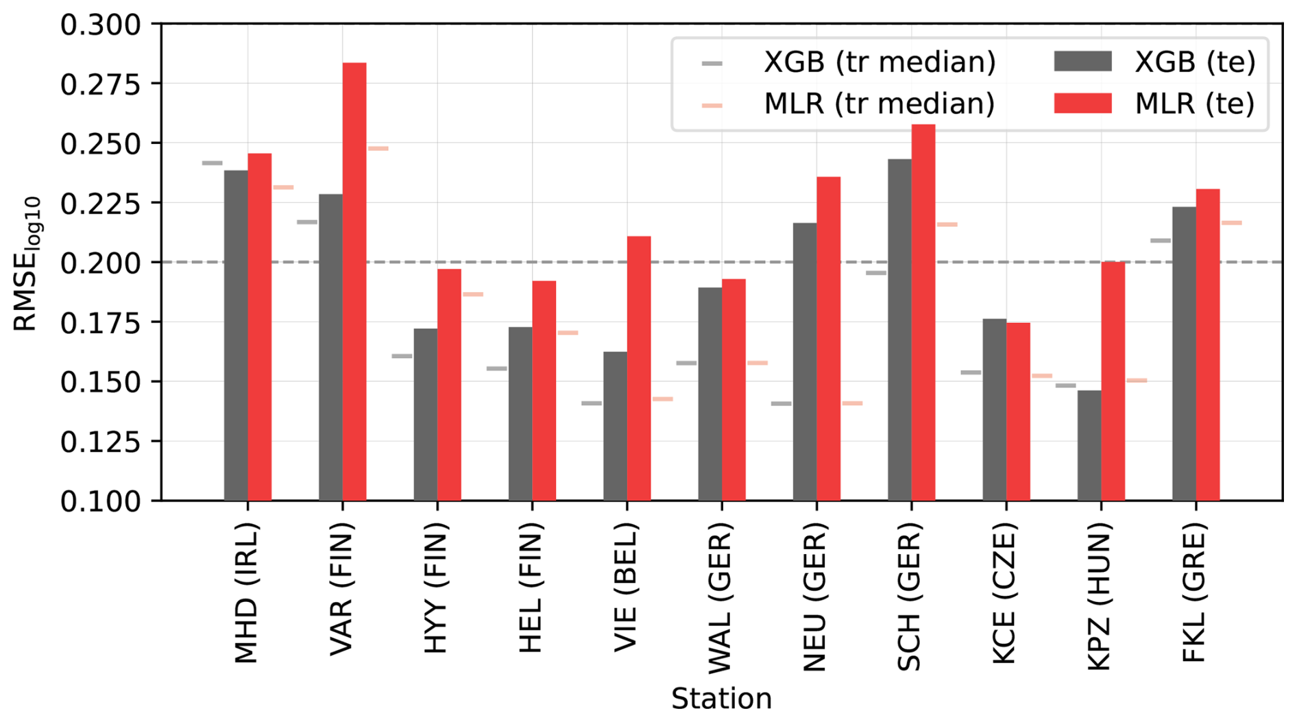
Figure 4 Comparison between the testing error (RMSE calculated for log₁₀-transformed concentrations) of the single-station ML models (ML models trained with data from one station) at each station with XGB and MLR machine learning models. The bars show the testing error for both models, and the lines indicate the median training errors corresponding to Fig. 3.

5.1.2 Assessing station-excluded and station-included model performance

We first looked at the performance of the station-excluded models, which were trained separately for each station. Figure 5 depicts the station-excluded N₁₀₀ estimates against the observed N₁₀₀ for all of the stations when no data from the target station were included in the training set. In practice, this means that, for each station, the estimated N₁₀₀ was produced with a different model and different validation set, and the results are presented in one figure. In contrast to the other instances where we used the station-excluded models, here, the estimates were not generated for all of the available data from the target station (Table 3). Instead, we used only around 200 d to have a comparable number of data points from all stations in the validation sets. The sampling method for these 200 d is explained in Sect. S3.

Figure 5 provides a rough indicator of how the global ML models would perform in locations not directly represented in the training set. Looking first at the MLR result (Fig. 5a), even when each station had been excluded from the training set, the station-excluded MLR models could produce the range of observed N₁₀₀ values from below 10 cm⁻³ to over 10⁴ cm⁻³. However, the station-excluded models still struggled with replicating the observations at the low concentrations, and, in general, 54 % of daily estimates and 15 out of 35 station median estimates fell outside the factor of 1.5 from observations.

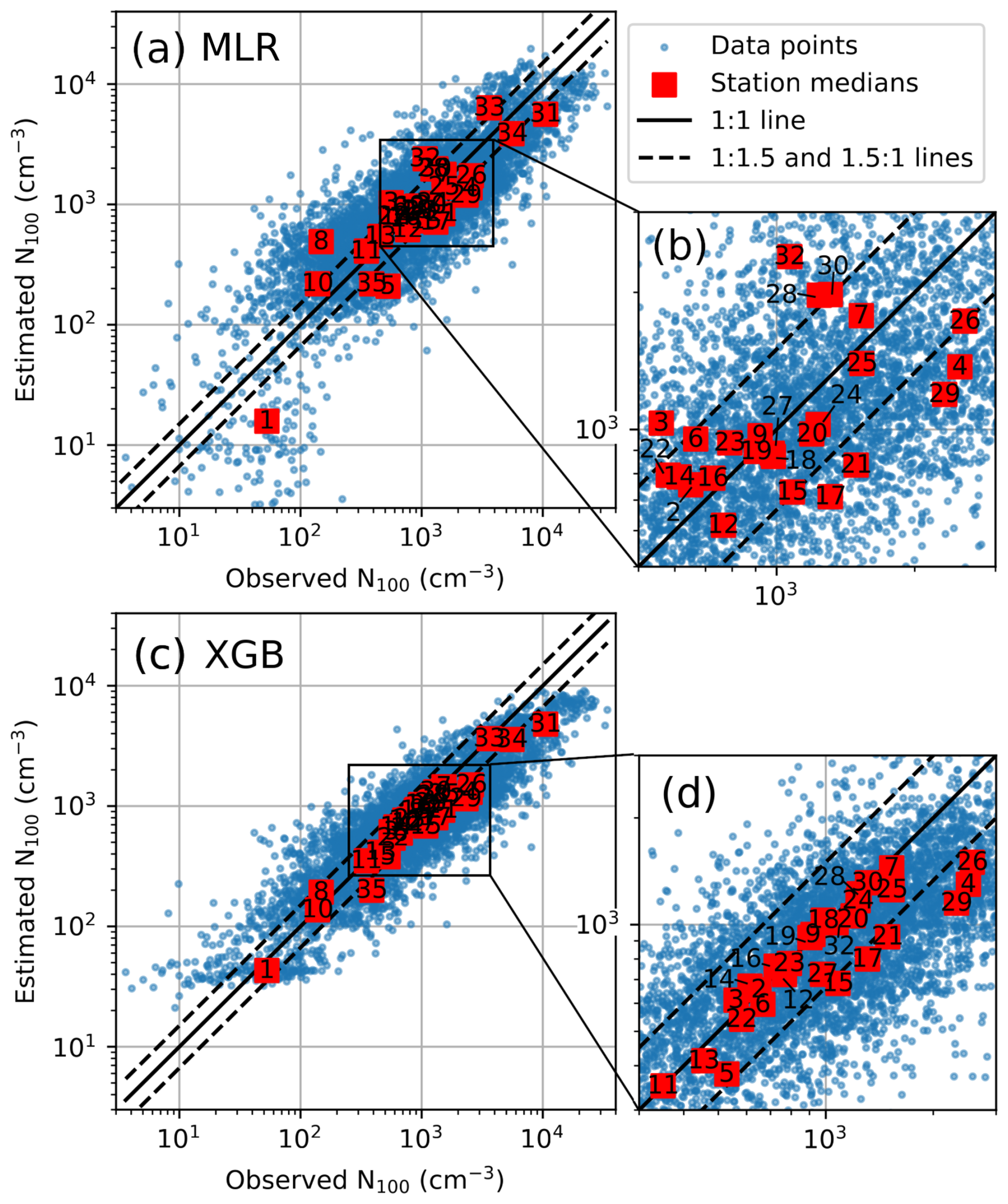
Figure 5 Comparison between observed and estimated N₁₀₀. The sampling of the data points shown in this figure is explained in Sect. S3. Panel (a) shows the result for station-excluded MLR models, and panel (b) shows a zoom-in. Panels (c)–(d) show the result and zoom-in for station-excluded XGB models. The daily values are indicated in blue, and station medians are indicated in red. The station medians are additionally marked with numbers which indicate the station, as listed in Table 1.

For the station-excluded XGB models (Fig. 5b), the station medians were better captured, with only nine station medians falling outside the 1.5-factor limit. The daily values were also captured slightly better, though, still, 48 % fell outside the factor of 1.5. The station-excluded XGB models also failed to reproduce extreme values: they could not produce values below 25 cm⁻³, systematically underestimated values above around 5000 cm⁻³, and could not produce values above 10⁴ cm⁻³. Overall, these results show that the XGB models tend to be slightly more precise and replicate the median values better, but MLR models are better at extrapolating to low and high concentrations, though they still struggle to capture extreme values.

Next, we analyzed in more detail the MLR and XGB station-excluded performance at different stations. To ensure that the training-error analysis (Fig. 6) was reliable, we first compared the training and testing errors against each other at the stations that had data after 2020 (Fig. S2). Because the target station had been left out of the training set in the station-excluded models, the main difference between the training and testing errors was that the training error was calculated with observations before 2020, and testing errors were calculated with observations after 2020, whereas the data before 2020 had also been used to optimize the ML models. Figure S2 shows that, for station-excluded models, the difference in training and testing errors was small, and we felt confident in drawing conclusions from the training error.

In terms of training error (Fig. 6), 25 out of 35 stations showed lower RMSE${}_{{\log }_{\mathrm{10}}}$ values for XGB compared to MLR, indicating generally better performance. However, MLR achieved equally good or better performance at 10 stations. Figure 6 also shows that the station-excluded performance varied depending on the station. The European stations typically had good or even excellent performance, probably because the N₁₀₀, different emissions, and meteorological conditions at many of the European stations were quite similar to each other. Even when the target station was left out from the training of the station-excluded model, there would still be at least one similar station in the training set. Conversely, stations with poor station-excluded performance might correspond to environments that did not have representation in the training set if the station was excluded from training.

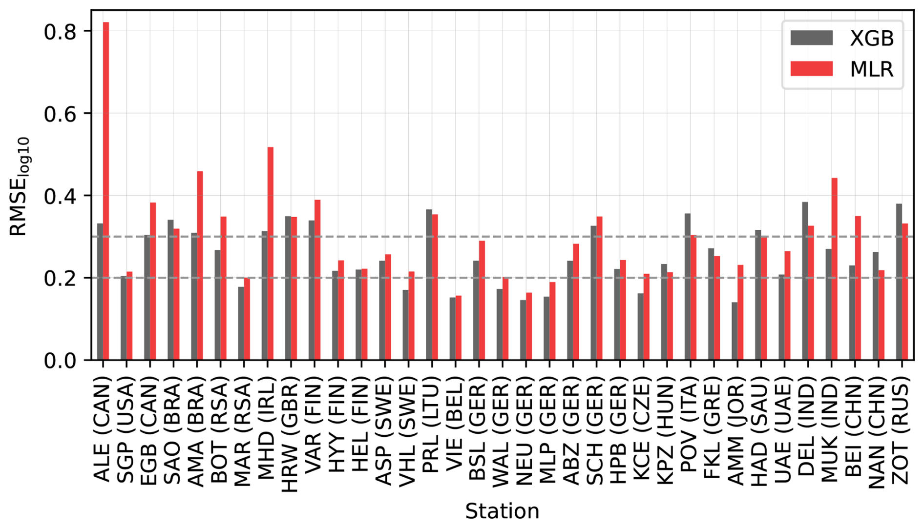
Figure 6 Comparison between station-excluded MLR and XGB model performance (RMSE calculated for log₁₀-transformed concentrations) at each station.

To investigate further this variation in performance, we analyzed the station-included models’ performance and compared them against the station-excluded models’ performance (Fig. S3). For the stations with excellent station-excluded performance (RMSE${}_{{\log }_{\mathrm{10}}}<$ 0.2), we noticed that the differences between the station-included and station-excluded model RMSE${}_{{\log }_{\mathrm{10}}}$ were small (below 0.01). This supports our interpretation that, for many European sites (Vielsalm, Belgium; Waldhof, Germany; Neuglobsow, Germany; and Melpitz, Germany, for both MLR and XGB models and Vavihill, Sweden, and Košetice, Czech Republic, for only the XGB model) and some other stations (Southern Great Planes, USA; Amman, Jordan; and Marikana, South Africa, for the XGB model), it did not matter whether the station had been excluded from the training because the other stations could still represent the excluded station during training.

Conversely, for many stations, the station-included models produced clearly better results than station-excluded models (Fig. S3). For the XGB model, these stations include Delhi, India; Hada al Sham, Saudi Arabia; São Paulo, Brazil; Po Valley, Italy; Zotino, Russia; Amazonas, Brazil; Nanjing, China; Värriö, Finland; and Alert, Canada. The better performance confirms that these stations have some unique characteristics, and, without their contribution, the XGB model could not capture the type of environment they represented. For example, when Delhi, India, which has the highest N₁₀₀ in our dataset, was excluded from the training set, the models could not replicate the high N₁₀₀ values. This led to underestimation and poor performance at the station (not shown).

The MLR models were less sensitive to whether station-specific data were included in training compared to the XGB models (Fig. S3). Because MLR uses linear predictor functions, adding a small number of new data points does not always affect the model performance, resulting in smaller differences between the station-included and station-excluded model versions. In contrast, any new data in the XGB models can alter the tree structure, affecting model performance. However, this also increases the risk of overfitting, which may reduce the XGB model’s ability to generalize outside the measurement stations.

5.1.3 Time series

Figure 7 compares the observed N₁₀₀ time series in 2013 to the estimated N₁₀₀ time series produced with the station-excluded and station-included models. The comparison allowed for a better understanding of the ML model behavior outside the measurement stations.

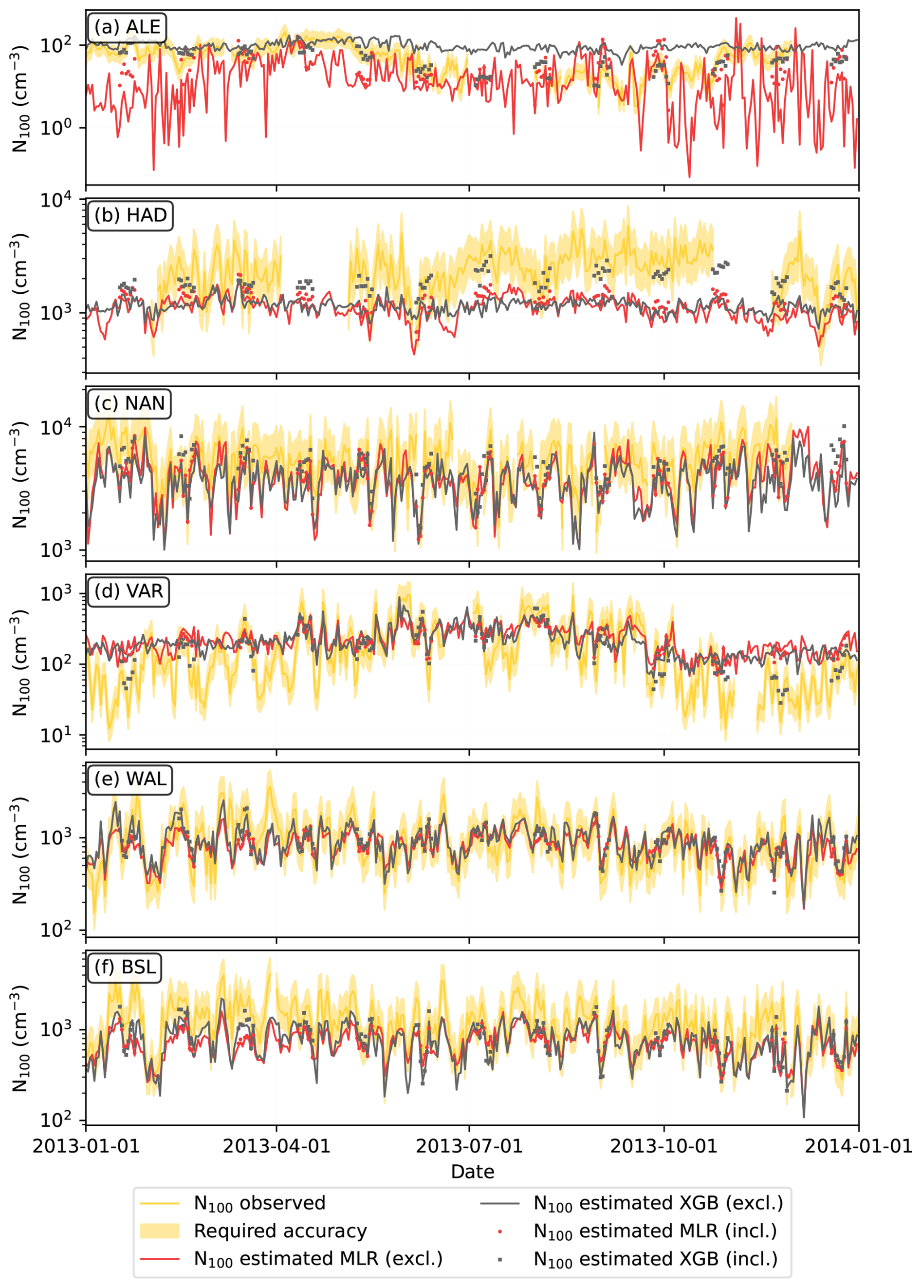
Figure 7 Comparison between observed and model-estimated N₁₀₀ time series for 2013 at selected stations. The required accuracy is within a factor of 1.5 from the observations based on Rosenfeld et al. (2014). Station-excluded estimates and station-included estimates are described in Table 3. Panels show the results for the stations at (a) Alert, Canada (ALE); (b) Hada al Sham, United Arab Emirates (HAD); (c) Nanjing, China (NAN); (d) Värriö, Finland (VAR); (e) Waldhof, Germany (WAL); and (f) Bösel, Germany (BSL).

In our dataset, Alert, Canada (ALE), was the sole representative of the extremely clean polar regions (Fig. 7a). When ALE was excluded from the training, none of the models performed well at that location, demonstrating the challenge of missing environmental types in the training set. However, when ALE was included in the training, the models, especially XGB, produced better estimates.

In Hada al Sham, Saudi Arabia (HAD), both station-excluded models underestimated N₁₀₀, whereas, among the station-included models, the MLR model showed some improvement, and the XGB model improved noticeably (Fig. 7b). The underestimation likely stems from the station’s complex surroundings, which include desert, sea, and a nearby hotspot of anthropogenic and biogenic activity (Hakala et al., 2019). While actual concentrations at the station can be high due to the hotspot, reanalysis data cannot resolve such sub-grid-scale variability, resulting in underestimated predictor values and low N₁₀₀ estimates. The station-included XGB model may still perform well if the predictors maintain a correlation with N₁₀₀, even when underestimated.

Nanjing, China (NAN), N₁₀₀ estimates were captured well, though they were mildly underestimated with the station-excluded models and the MLR station-included model (Fig. 7c). The station-included XGB model produced slightly better results. It is possible that specific environmental characteristics in Nanjing contribute to underestimation when using reanalysis data to estimate N₁₀₀.

In Värriö, Finland (VAR), the models performed well during summer, but the station-excluded models overestimated the low concentrations during winter (Fig. 7d). While the MLR station-included model did not yield notably better results than station-excluded models, the XGB station-included model successfully captured the winter periods as well. In general, low concentrations tend to be quite difficult for our ML models to capture, but the station-included XGB model likely succeeds in capturing them because the tree structure allows it to fit more closely to any included training data.

Waldhof, Germany (WAL), a typical European station, was well represented by other stations in the dataset (Fig. 7e). Consequently, even when WAL was excluded from training, the estimated N₁₀₀ time series still aligned closely with the observations. Including data from Waldhof in the training set did not enhance the results. In contrast, in Bösel, Germany (BSL) (Fig. 7f), another central European station, both the station-included and station-excluded models systematically underestimated N₁₀₀, although the daily variations were captured well. Birmili et al. (2016) noted that the total particle concentrations in Bösel were higher than at the other rural German sites.

5.2 Global ML models and N₁₀₀ fields

5.2.1 Feature importance

Moving on to the final global ML models, Fig. 8 shows the importance of different features in MLR_global and XGB_global. The two most important variables in both ML models were the black carbon aerosol (BC) mixing ratio and the organic matter aerosol (OM) mixing ratio. In MLR_global, these variables were hydrophilic, whereas, in XGB_global, they were hydrophobic. However, we should not conclude that these variables were truly the most important ones. Due to the underlying dynamics of the CAMS dataset, BC and OM mixing ratios were highly correlated (Fig. S4), as were the hydrophilic and hydrophobic mixing ratios (not shown). Such strong correlations between variables can pose challenges for ML models (e.g., Kuhn and Johnson, 2013). In the MLR_global model, we observed an unexpected result: instead of assigning positive coefficients to both variables, it assigned a high positive coefficient to the hydrophilic BC mixing ratio while giving the hydrophilic OM mixing ratio an approximately equally high negative coefficient. This suggests that the MLR_global model may have overestimated the influence of hydrophilic BC and then counterbalanced this by assigning a negative coefficient to hydrophilic OM. Typically, their combined effect on N₁₀₀ was quite small. However, if the BC and OM mixing ratios are less closely linked in certain locations or during certain time periods, this imbalance could significantly affect the predicted N₁₀₀ concentrations. To explore this further, we analyze their relationship in Sect. S5 (Fig. S5).

Aside from the BC and OM mixing ratios, the most important variables influencing the ML models were sulfate aerosol, ammonia, carbon monoxide, and sulfur dioxide mixing ratios followed by temperature (Fig. 8). Since most of these variables are primarily associated with anthropogenic sources, it is unsurprising that, in the MLR_global model, they exhibited a positive relationship with N₁₀₀ concentrations, meaning that an increase in their concentrations led to an increase in N₁₀₀.

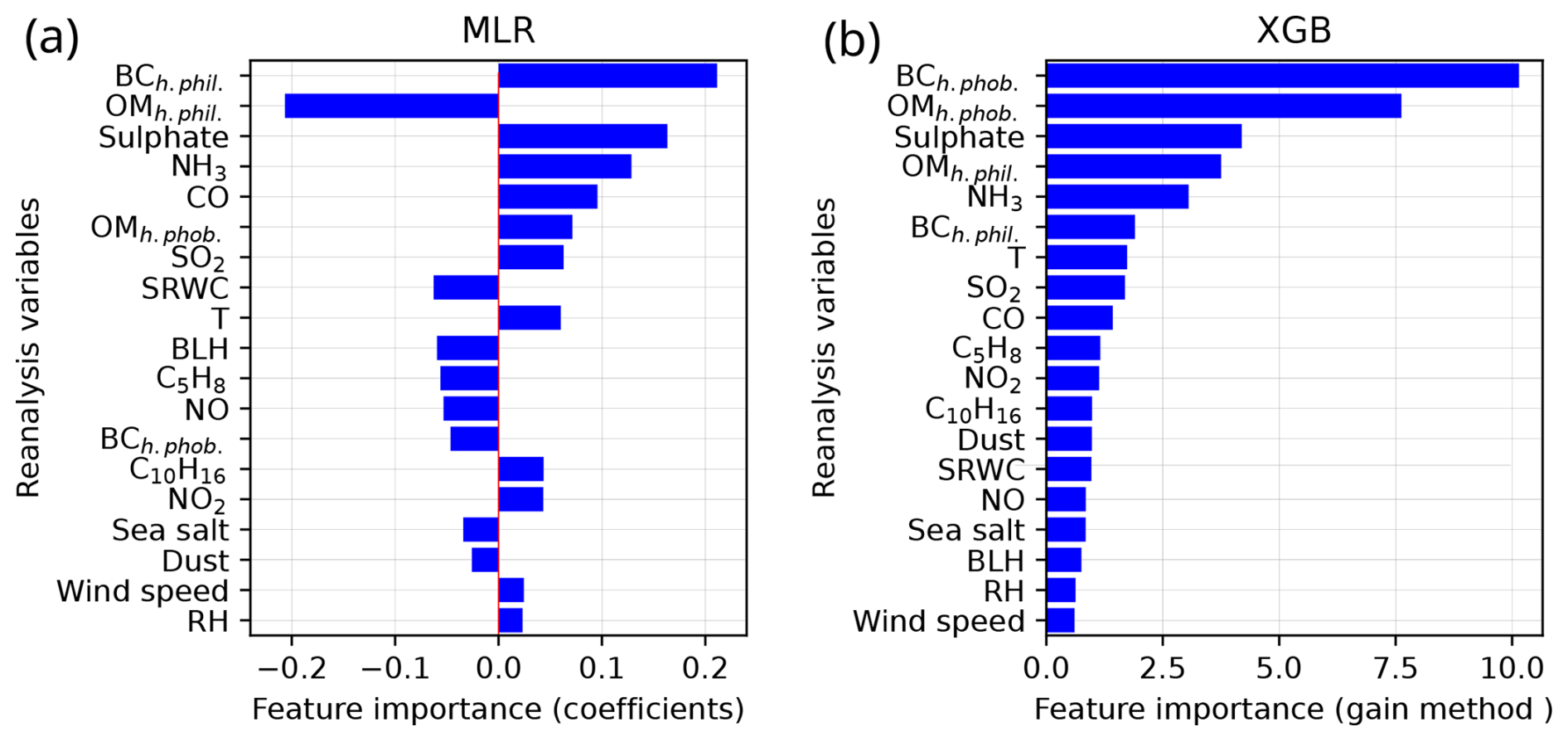
Figure 8 The global ML model feature importance in descending order. Panel (a) shows MLR_global model feature importance based on MLR coefficients. Panel (b) shows XGB_global feature importance based on the gain method.

In contrast, the variables more linked to the natural processes tended to have lower importance and showed both positive and negative coefficients in the MLR_global model. Some coefficients aligned directly with the expected physical processes. For example, the relationship between specific rainwater content (SRWC) and N₁₀₀ is negative because rain removes aerosol particles from the air. Similarly, the negative coefficient for boundary layer height (BLH) reflects how a larger daily mean BLH dilutes N₁₀₀ by mixing it into a larger volume of air.

Additionally, there were variables that have physically meaningful coefficients, but the interpretation is more nuanced, such as in the case of the sea salt aerosol mixing ratio. A higher concentration of sea salt aerosol should result in a higher N₁₀₀ concentration. However, because a higher sea salt aerosol concentration often coincides with the arrival of clean marine air masses, MLR_global interprets the relationship to be negative. This is a meaningful interpretation over continental areas, but over oceans (which were not represented in our training set), it would fail to capture the true relationship between sea salt aerosol concentration and N₁₀₀. Moreover, a high sea salt concentration in the sub-0.5 µm size is probably accompanied by a high supermicron sea salt aerosol concentration, which gives few additional primary CCN but may substantially suppress secondary CCN formation by acting as a sink for low-volatility vapors and sub-CCN-sized particles. A similar phenomenon can explain the negative coefficient of the sub-0.55 µm dust aerosol.

Finally, there were variables for which the MLR coefficients might not have been able to capture the physical processes. One of these was temperature, which may have a complex relationship with N₁₀₀ depending on the location. For example, in many parts of the world, temperature can be associated with increased volatile organic compound (VOC) emissions, which leads to a larger number of aerosol particles growing to the accumulation-mode size range (Paasonen et al., 2013). This effect has a strong correlation with isoprene (C₅H₈) and terpene (C₁₀H₁₆) emissions, and MLR_global may struggle with variables with strong correlations. However, a negative coefficient being assigned for C₅H₈ mixing ratios but a positive coefficient being assigned for C₁₀H₁₆ mixing ratios and temperature agrees with several studies suggesting that isoprene likely inhibits the secondary aerosol formation and growth of particles to N₁₀₀ sizes (Lee et al., 2016; Heinritzi et al., 2020). Additionally, natural VOC emissions may be suppressed during the hottest days in many environments. On the opposite side of the temperature spectrum, cold temperatures can also lead to higher N₁₀₀ concentrations due to heating-related residential biomass combustion, which consequently increases aerosol and aerosol precursor emissions. The MLR_global cannot capture these complex patterns directly but may attempt to do it indirectly via correlating variables. This may also explain other counterintuitive coefficient values, such as NO₂ having a positive coefficient and NO having a negative coefficient.

5.2.2 The global N₁₀₀ fields

Figure 9 shows the annual mean N₁₀₀ fields in 2013, calculated by averaging the daily N₁₀₀ estimates – see Fig. 9a for MLR_global and Fig. 9b for XGB_global. Both models estimated the highest N₁₀₀ in South Asia and East Asia and the lowest N₁₀₀ in remote locations such as polar areas and deserts.

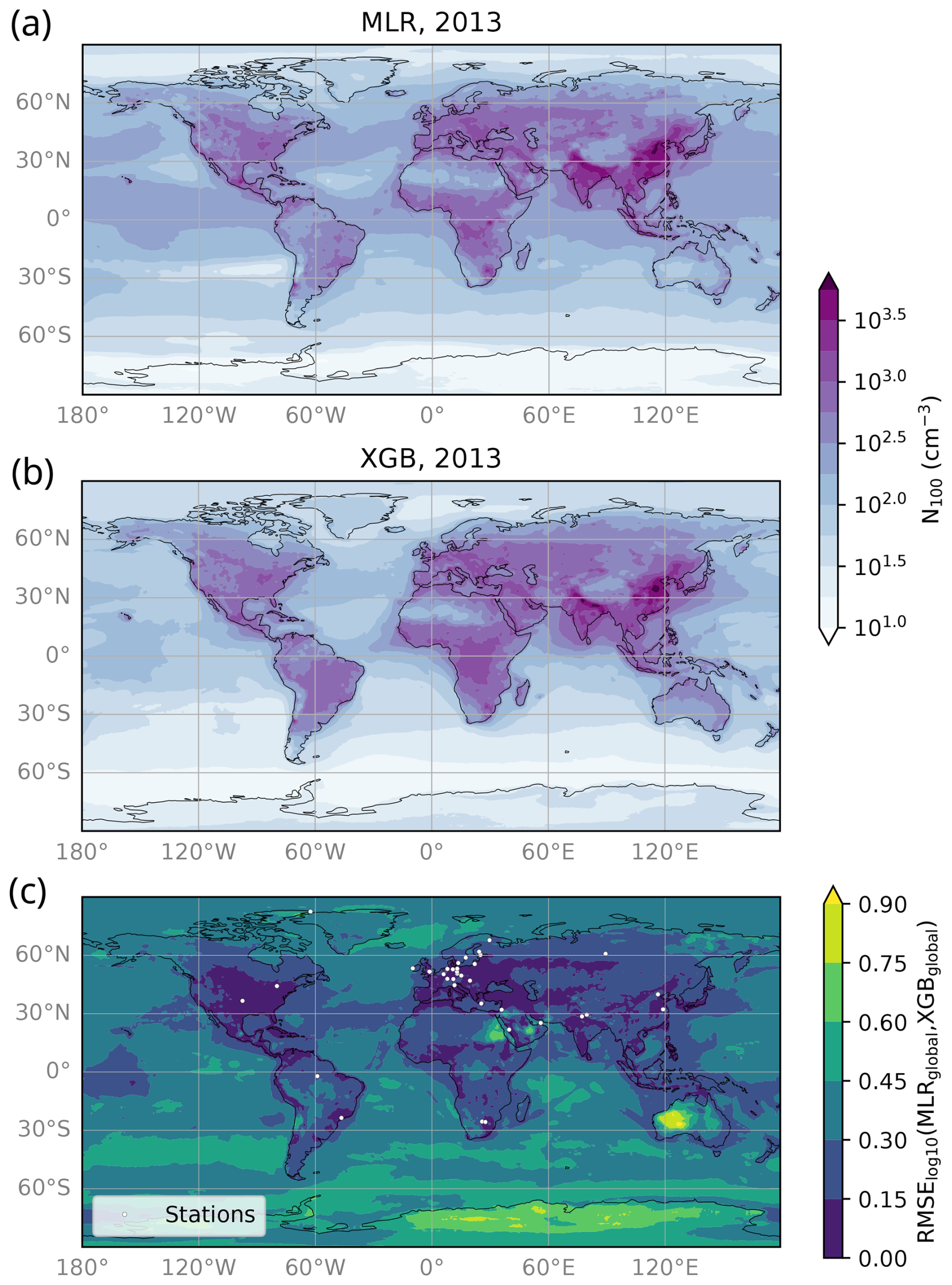
Figure 9 The estimated annual average N₁₀₀ for 2013 (a) with the MLR_global model and (b) with the XGB_global model. The models were trained with all available measurement data and all measurement stations. Panel (c) shows the comparison of estimated daily N₁₀₀ for 2013 from MLR and XGB models, where the color scale shows the root mean squared error between the log₁₀-transformed N₁₀₀ estimates. The smaller the RMSE value, the better the models agree. RMSE values below 0.3 indicate that the models agree well, and values below 0.15 indicate that the models agree very well.

The comparison between MLR_global and XGB_global N₁₀₀ fields for 2013 is shown in Fig. 9c. Overall, the ML models produced similar values across most continental areas, particularly in large parts of Europe and North America, though the XGB model generally yielded slightly higher estimates. Additionally, the results agreed well (RMSE${}_{{\log }_{\mathrm{10}}}<\mathrm{0.15}$) near most measurement stations, as well as in more densely populated areas (Smith, 2017, 2023), even in regions without in situ measurements. This pattern is evident in the most populated areas in the Middle East, southern Siberia, and Central Asia. In South America and Africa, the model agreement was also better in the more populated regions. However, the limited number of measurement stations in these continents may affect the results because not all populated regions showed strong agreement between the models. A similar trend was observed in South and East Asia. While these regions are, overall, very densely populated, only the most highly populated areas exhibited strong agreement, which may also relate to the distribution of measurement stations. Although the agreement between models does not confirm accuracy against measurements, it suggests consistency between the models. This consistency is likely because these regions are well-represented in the model training, either directly through a nearby station or indirectly because most of the stations in our dataset are located in anthropogenically influenced areas.

The models diverged in several regions (Fig. 9c), particularly over remote or clean continental environments such as Antarctica, the Australian deserts, the eastern Sahara Desert, and parts of the Middle East (RMSE${}_{{\log }_{\mathrm{10}}}>\mathrm{0.60}$). In the latter two regions and some mid-latitude marine regions, the difference appeared to stem from low NH3 values (Fig. S6), which led MLR_global to generate lower N₁₀₀ estimates. Other continental areas with smaller but still considerable discrepancies (0.30 < RMSE${}_{{\log }_{\mathrm{10}}}<\mathrm{0.45}$) included parts of South America, particularly the Amazon Rainforest; the Congo Rainforest; and some regions in Africa, including the Kalahari Desert, where the MLR_global model consistently predicted lower N₁₀₀ values than XGB_global. Additionally, there were some hotspots where MLR_global produced clearly higher N₁₀₀ estimates compared to XGB_global. The divergence likely stems from different responses to anthropogenic variables in the MLR_global and XGB_global models. While the anthropogenic variables were important in both models, the linear relationship between the variables and N₁₀₀ in the MLR model seems to cause underestimation in low N₁₀₀ values – common in clean or remote environments. The XGB model did not exhibit this behavior, possibly due to its non-linear nature. However, in some locations, the lower N₁₀₀ estimates from the MLR model appear to be more accurate than those from XGB. For example, in Alert, the station-excluded MLR model captured certain low N₁₀₀ values better than the station-excluded XGB model.

Notable differences also emerged over the oceans (Fig. 9c), which are poorly represented in our training set. In these regions, MLR_global typically produced much higher N₁₀₀ estimates than XGB_global. However, the models showed better agreement in continental outflow areas, such as in the northwestern Pacific Ocean and along major shipping routes, likely due to their anthropogenic influence, which makes them better represented in the model training.

The testing errors for MLR_global and XGB_global models at stations with 2020–2022 observations are shown in Fig. 10. These global ML model errors aligned with previous analyses, such as the station-excluded testing errors (also in Fig. 10), with performance varying by location and the XGB model generally outperforming MLR_global. The most notable differences between global and station-excluded model performance occurred at Mace Head (Ireland), Värriö (Finland), and Schauinsland (Germany). In all of these locations, the global XGB models performed better. This improvement was likely due to the frequent low concentrations at these stations, which are challenging to capture without training representation from the target station. In Mace Head, these low concentrations were related to clean air masses coming from the ocean; in Värriö, they were associated with clean winter periods; and in Schauinsland, they were associated with times when the measurement station was above the boundary layer.

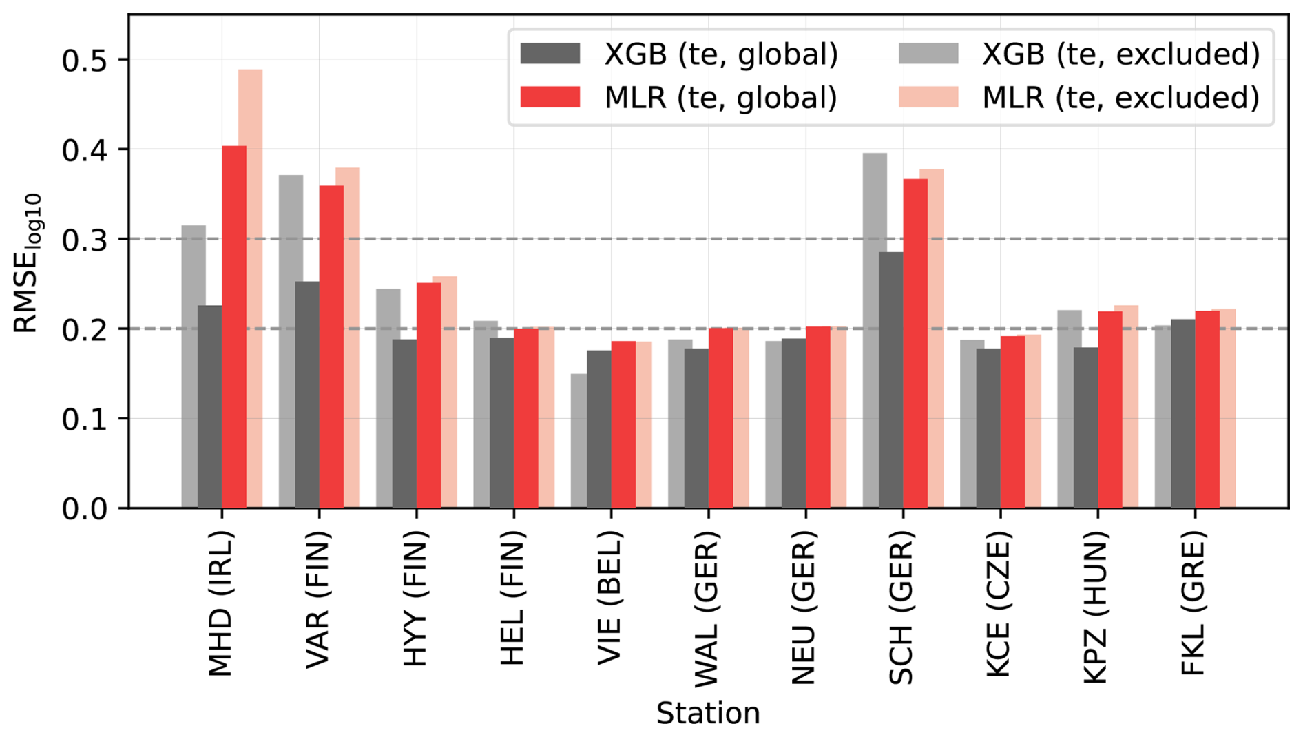
Figure 10 The comparison between MLR_global and XGB_global testing errors (RMSE calculated for log₁₀-transformed concentrations) and station-excluded model testing errors (corresponding to Fig. 6) for the stations that had N₁₀₀ measurements for 2020–2022.

5.3 Interpreting results from different ML models

By evaluating model performance across the intermediate models (single-station models, station-included models, and station-excluded models) and global models, we identified three cases where our models struggled to capture N₁₀₀ accurately. Figure 11 presents a comparison of the RMSE${}_{{\log }_{\mathrm{10}}}$ medians from the CV analyses for single-station models, station-included models, and station-excluded models (the version directly comparable to station-included models, as shown in Table 3).

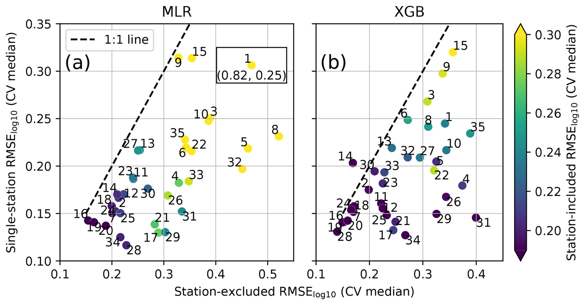
Figure 11 The comparison between the medians of cross-validation (CV) results from single-station and station-excluded models, colored with results from the station-included model, for (a) MLR and (b) XGB. The numbers correspond to stations as listed in Table 1. In panel (a) one data point (Alert, Canada, 1) was outside figure limits and is indicated separately in the figure with coordinates.

Firstly, our models struggled with capturing N₁₀₀ at certain stations, even when using single-station models (Fig. 11). While the single-station estimates performed well at most stations, two stations had poor performance (RMSE${}_{{\log }_{\mathrm{10}}}>\mathrm{0.3}$). Additionally, at stations with RMSE${}_{{\log }_{\mathrm{10}}}$ values between 0.2 and 0.3, certain conditions or characteristics may still be difficult for the single-station models to capture, lowering the performance, even though, overall, the RMSE${}_{{\log }_{\mathrm{10}}}$ values are acceptable. Notably, the stations with high single-station RMSE${}_{{\log }_{\mathrm{10}}}$ values often continued to exhibit lower performance in the other intermediate models, suggesting that these locations are inherently difficult to capture with our method (Fig. 11).

Several factors may explain these difficulties. Our dataset may lack key reanalysis variables necessary for accurately estimating N₁₀₀ in these environments. Reanalysis data may also contain uncertainties or struggle to resolve sub-grid-scale processes crucial for N₁₀₀ estimates. Additionally, the non-linear interactions between predictor variables and N₁₀₀ may not be fully captured by our ML models due to either inherent model constraints or the limited size of the training dataset. Among our datasets, both stations where single-station model RMSE${}_{{\log }_{\mathrm{10}}}$ values exceeded 0.3 (Harwell, United Kingdom, and Preila, Lithuania) had relatively short measurement time series. Furthermore, Xian et al. (2024) reported that the CAMS reanalysis AOD differs from the AERONET AOD in areas near Preila. Their observation suggests that there may be persistent sub-grid-scale variability in aerosol concentrations around the site, which could be contributing to model inaccuracies.

The second challenge our ML models faced was a decline in station-included model performance compared to the single-station models. While we expected some decrease due to the added complexity of incorporating multiple locations, the station-included performance declined notably at some stations. The decline was particularly evident in the MLR models, where, at 13 stations, the station-included model RMSE${}_{{\log }_{\mathrm{10}}}$ values were over 1.5 times higher than single-station model RMSE${}_{{\log }_{\mathrm{10}}}$ values (Fig. S7a). For the XGB models, the station-included performance was notably worse than single-station performance in Schauinsland (Germany) and possibly in Bösel (Germany) and Annaberg-Buchholz (Germany) (Fig. S7b). This weaker performance may arise from variable–N₁₀₀ interactions that differ from other stations. Since the models – especially the MLR model – struggle to capture conflicting variable–N₁₀₀ relationships, stations with unique interactions relative to the rest of the dataset tend to experience the largest performance decline from single-station models to station-included models. The unique interactions that lead to performance decline may arise not only between observed N₁₀₀ and real aerosol, gas, or meteorological variables but also artificially between observed N₁₀₀ and CAMS variables distorted by uncertainties. One example of such artificial interaction is the sub-grid-scale variability-related underestimation seen in MLR estimates at Hada al Sham, as discussed in Sect. 5.1.3.

Conversely, at least at one station (Vavihill, Sweden), the station-included XGB model outperformed the single-station XGB model (Fig. S7b). One explanation for this improvement is that Vavihill has a relatively short measurement series in our dataset, which limited the single-station performance. However, in station-included models, Vavihill’s data may be supplemented by the data of other similar stations in our dataset, improving the performance.

Thirdly, our models struggled in locations that were not well-represented in our training data. While single-station and station-included models, which incorporated station-specific data, generally captured N₁₀₀ at least moderately well (RMSE${}_{{\log }_{\mathrm{10}}}<\mathrm{0.3}$), station-excluded models performed notably worse at certain sites – even when the station-included performance was excellent (RMSE${}_{{\log }_{\mathrm{10}}}<\mathrm{0.2}$) (discussed in more detail in Sect. 5.1.2). Figure 11 illustrates this pattern, especially for the XGB models: when the XGB station-included performance was excellent (RMSE${}_{{\log }_{\mathrm{10}}}<\mathrm{0.2}$), the station-excluded performance varied widely, ranging from excellent (RMSE${}_{{\log }_{\mathrm{10}}}<\mathrm{0.2}$) to poor (RMSE${}_{{\log }_{\mathrm{10}}}>\mathrm{0.3}$). If both station-included and station-excluded performances were excellent, it indicated that N₁₀₀ in these stations could be captured well even without their own data in the training set because similar stations in our dataset provided sufficient representation. Conversely, as station-excluded RMSE${}_{{\log }_{\mathrm{10}}}$ increased, it was suggested that incorporating station-specific data became increasingly important for accurate estimates. This effect was particularly notable in environments with high N₁₀₀ concentrations compared to the other stations.

Our cross-validation indicated that our training set best represents European urban or rural environments influenced by human activity and similar anthropogenically influenced environments. Even when evaluating the global ML models with a holdout set containing data from the period of 2020–2022 (Fig. 10), the models performed well in capturing N₁₀₀ at the European stations. The global model comparison gives similar results, showing that the models tend to agree in Europe but also in other populated areas.

5.4 ML model limitations

While our results demonstrate promising performance across many environments, the findings from Sect. 5.3 highlight that model accuracy depends strongly on the availability and representativeness of training data. In other words, different limitations in the N₁₀₀ measurements and reanalysis data cause limitations in the ML models. While Sect. 5.3. touched upon these issues, here, we discuss them further.

For the N₁₀₀ measurements, the main challenge is data availability. To train ML models that capture diverse environments and meteorological conditions, we require a broad dataset that covers a wide range of locations and time periods. In an ideal case, the dataset would represent environments with different natural and anthropogenic emission levels extending from low to high global extremes, as well as a wide spectrum of different anthropogenic to natural contribution ratios. The global distribution of long-term datasets, reflected by measurement stations utilized in this study, is clearly biased towards continental, anthropogenically influenced, and European environments. Thus, the performance of our global ML models is expected to be worse in marine and tropical environments, as well as in the Southern Hemisphere and in polar regions. In addition, ideally, we would have at least 5 years of data from each station. This would allow for the division of data into training, validation, and holdout sets, with at least one full seasonal cycle in each set and multiple cycles in the training set. Since environmental conditions and aerosol concentrations vary between years, such a dataset would enable ML models to generalize better and learn from a broader range of conditions, resulting in more robust estimates. Unfortunately, our current dataset lacks full seasonal coverage at some stations, which makes it harder for the ML models to accurately capture station-specific and global trends. This emphasizes the need for continuous long-term observations.

Another challenge with in situ measurements is potential measurement errors that may remain after filtering. These errors can propagate into the ML models, affecting overall accuracy. Additionally, because our method relies on ground-level N₁₀₀ measurements, the ML models can only produce ground-level N₁₀₀ estimates and do not provide vertical profile information, which is needed for certain applications. For example, when studying aerosol–cloud interactions, CCN concentrations near or above the cloud base are particularly important (Quaas et al., 2020). While the ground-level aerosol concentrations represent the cloud-level concentrations in well-mixed boundary layers, where surface and cloud base conditions are coupled, they do not reflect cloud-level concentration under decoupled conditions (Su et al., 2024).

Regarding reanalysis data, CAMS and ERA5 are subject to various uncertainties that can affect the performance of our ML models. Block et al. (2024) provide a detailed overview of uncertainties in CAMS aerosol variables, including limited satellite retrievals in polar regions; omissions such as volcanic activity; and specific volcano-related biases around sites like Mauna Loa (Hawaii, USA) and Altzomoni (Mexico), both of which emerge as hotspots in our MLR model results. Additionally, CAMS currently excludes nitrate aerosol mixing ratios (Inness et al., 2019a) and applies a simplified partitioning scheme for hydrophilic and hydrophobic BC and OM based on emission fractions and a time-dependent conversion rate (Rémy et al., 2022). We should also note that the relations between N₁₀₀ and OM or BC in our ML models are likely to be affected by the apparent challenges by CAMS in predicting the overall concentration levels of OM (Amarillo et al., 2024) or past changes in BC concentrations over areas such as China (Li et al., 2024).

For gas compounds, CAMS variables assimilated with satellite retrievals – such as CO and NO_x – have been evaluated in studies by Inness et al. (2019a) and Langerock et al. (2024). In contrast, variables not assimilated with satellite data are less thoroughly investigated, and their uncertainties likely vary notably across variables and regions. Although we do not explicitly assess the impact of these CAMS uncertainties on our ML model, they are expected to introduce errors into our global N₁₀₀ fields.

Moreover, integrating gridded reanalysis data with single-point N₁₀₀ measurements can introduce challenges at the stations located in grid cells with sub-grid-scale variability in emission sources, meteorology, and topography. Because reanalysis data represent grid cell averages, these may not capture the true predictor variable concentrations at the measurement site, even if the reanalysis data are interpolated to the exact station location, leading to uncertainties in the model’s learned relationships. This discrepancy, along with other CAMS uncertainties, may partly explain the poor performance observed at some stations, even when using single-station models.

6 Summary and conclusions

Observation-based data on global accumulation-mode particle number concentrations (N₁₀₀) are essential for assessing global CCN concentrations and their climate impacts, as well as for evaluating Earth system models. According to Rosenfeld et al. (2014), reducing uncertainties in aerosol–cloud interactions requires capturing global CCN concentrations within a factor of 1.5 of true values. In this study, we developed a method for generating global N₁₀₀ fields using a combination of in situ measurements, reanalysis data, and machine learning. For evaluating ML model performance at measurement stations and outside of them, we applied cross-validation to several intermediate models. We also trained global ML models on all available data and generated daily global N₁₀₀ fields for 2013.

We found that, at least in a simple setting, such as in estimating the N₁₀₀ at a specific location with the single-station models, our method yields good results. This is especially true for the XGB model. However, some stations were more challenging to capture, possibly due to an insufficient number of data points, missing crucial reanalysis variables, or inadequate representation of sub-grid-scale variability in concentrations and other reanalysis data uncertainties. Additionally, ML models – particularly the MLR model – may struggle to capture the non-linear interactions between N₁₀₀ and the reanalysis variables at these stations. The stations where single-station models struggled remained challenging for all types of intermediate models.

Addressing these limitations is challenging, but future work could explore incorporating additional variables, for example, accounting for a station’s position relative to the top of the boundary layer, which might help improve ML model performance in high-altitude environments by allowing models to recognize when stations are above it. Additionally, refining the grid selection scheme could improve accuracy at stations where sub-grid-scale variability causes the reanalysis data to misrepresent local conditions. Comparing observed concentrations of key predictor variables with their reanalysis counterparts can help identify discrepancies. If significant differences emerge, selecting a nearby grid cell that better represents the measurement station – such as choosing a land-only grid cell instead of one that includes both land and ocean – may enhance model performance.

Our primary approach for evaluating ML model performance in areas without observations was cross-validation using station-excluded models. For each station, we trained an ML model without station-specific data and assessed how well the model reproduced the station’s observations. The analysis of these station-excluded models revealed that model performance largely depended on whether the training set contained stations with similar characteristics. This analysis suggests that our global ML models can generalize beyond measurement stations if the environments or conditions resemble the stations in our training set.

For the final global ML models, we investigated feature importance and model interpretation in more detail. Both global ML models identified sulfate aerosol and ammonia, carbon monoxide, and sulfur dioxide mixing ratios as the most important variables. BC and OM mixing ratios were also indicated as important, though their combined contribution was likely to be minor. We used the feature importance to interpret some of the model behavior of the MLR model. We noticed that some variables, such as sea salt aerosol, were represented in ways that do not apply universally across locations and conditions, potentially impacting ML model performance.

The comparison between MLR_global and XGB_global fields for 2013 revealed that the models agreed better in Europe, North America, and many other densely populated and anthropogenically influenced regions, including the most densely populated areas in South America, Africa, the Middle East, southern Siberia, and South and East Asia. These areas were likely to be better represented in the training data, making the ML models potentially more reliable in those regions, though we cannot be certain. Conversely, the ML models showed greater disagreement in remote areas, such as deserts, polar regions, rainforests, and oceans, suggesting that these environments may be more challenging for the models to capture. Our analysis did not indicate whether the MLR or XGB model, if either, performed better in these regions.

Overall, both the MLR and XGB models have their advantages and disadvantages, and our analysis could not definitively determine which model should be used for generating global N₁₀₀ fields. XGB generally performed better and was also able to capture N₁₀₀ in some unique conditions where the MLR model could not. However, in many locations, the MLR model produced equally good results. Additionally, MLR is less prone to overfitting and can produce better estimates when operating outside the range of N₁₀₀ values in the training set. The MLR model also offers greater interpretability as its variable coefficients can help identify areas where the model is likely to fail.

Our approach produces valuable results, even though our estimates did not fully meet the accuracy threshold suggested by Rosenfeld et al. (2014). At locations outside the training set, only 9 out of 35 stations had at least one ML model with RMSE${}_{{\log }_{\mathrm{10}}}$ values below 0.2, meaning that, in most locations, fewer than 70 % of daily N₁₀₀ concentration estimates fell within a factor of 1.5 of observations. Still, our method provides useful insights and enables global N₁₀₀ estimation where direct observations are unavailable. It complements other observation-based methods, such as satellite-derived approaches or the method outlined in Block et al. (2024) and can be used to evaluate purely model-driven results. A key advantage of our method is that it is directly constrained with in situ measurements of N₁₀₀ rather than relying solely on observations via data assimilation. Although our global N₁₀₀ fields were produced for 2013, the global N₁₀₀ time series can be extended to any period covered by CAMS data (currently 2003–2023). Moreover, this methodology could be applied to estimate other atmospheric variables with available in situ measurements and corresponding reanalysis data. However, it should be noted that ML models trained with observational data as the target variable cannot be expected to represent these variables reliably in too-distinct conditions – determining pre-industrial or future N₁₀₀ cannot be done based on present-day observations.

Improving and better evaluating the performance and reliability of the global MLR and XGB models in different environments and conditions will require additional data. We hope future research investments and collaborations will provide access to a wider long-term measurement dataset, extending especially towards marine, tropical, Southern Hemisphere, and polar areas that are underrepresented in the current study. Although adding new data from such measurement stations does not provide a global reliability estimate, it will allow us to improve and assess the model performance in new environments and conditions with unseen data. Including longer datasets from stations already part of this study will also improve the models due to capturing more variability in the atmospheric conditions at these sites. With the larger measurement dataset, it would be beneficial and straightforward to retrain the global ML models with the method described in this study. We could also explore using shorter datasets, such as measurement campaign data, for testing the models. While these datasets are too short for model training, they could enrich the holdout set by introducing environments that lack long-term measurements.